This computational essay explores the predictive accuracy of three models: non-linear model fits, state space models, and neural nets. The essay takes you on a journey from simple modeling techniques to discover the advantages of these techniques in a world where neural nets are gaining popularity. It is important to note that these modeling techniques are often used in conjunction with each other. However, for the purpose of comparing the models, they will be considered independently.
Introduction
Introduction
In[]:=
WordCloud[WikipediaData["Mathematical Modeling"]]
Out[]=
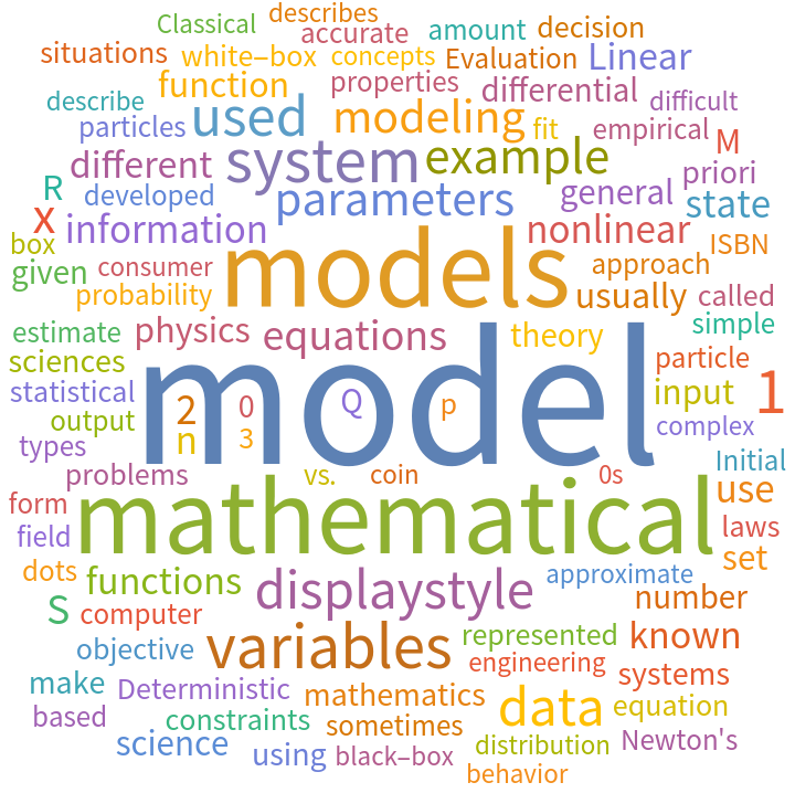
The purpose of this essay is to introduce a highly significant discussion. The emergence of machine learning has brought about groundbreaking advancements. However, have we thoroughly analyzed each technique in terms of their predictive power relative to one another? This essay aims to compare two crucial techniques: State-Space Models, specifically those employing the Kalman filter, and Neural Networks, which represent a more contemporary approach.
Data
Data
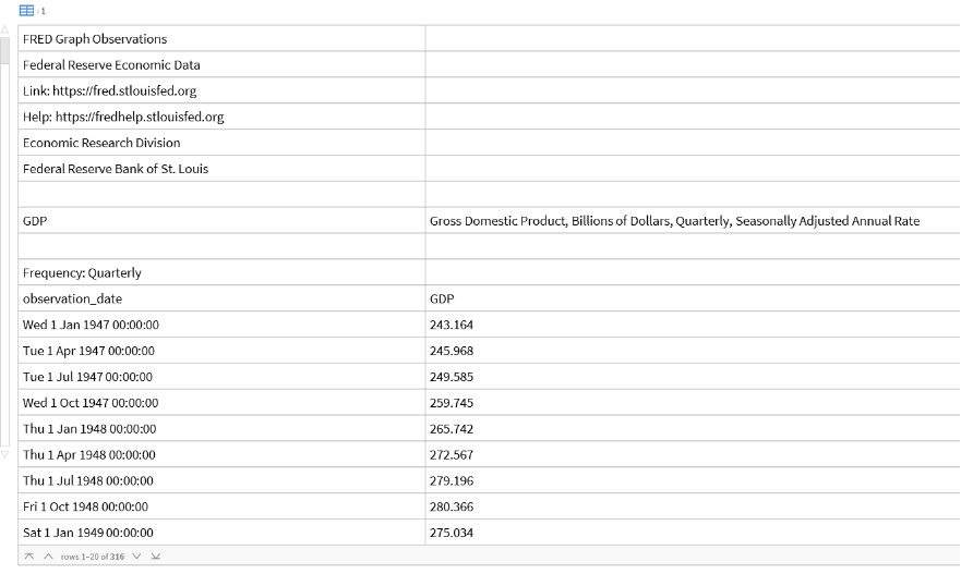
The data that will be used in this computational essay is the Federal Reserve of Economic Data (FRED) Real Gross Domestic Product data from 1947 to 2023.
data=Import["C:\\Users\\ali12\\Downloads\\GDP.xls"];preprocessedData=data/.Null->"";Dataset[preprocessedData]
In[]:=
gDPdataIcon=Iconize[preprocessedData,"GDPData"]
Out[]=
Splitting the Data into Train and Test Sets
Splitting the Data into Train and Test Sets
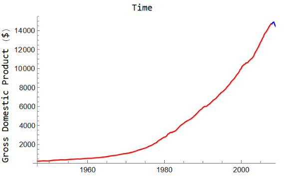
In this context, we will employ Mathematica to partition the dataset into separate testing and training sets. This division serves the purpose of evaluating the predictive capabilities of our models and safeguarding against the occurrence of overfitting.
whole=preprocessedData;{trainer,tester}=ResourceFunction["TrainTestSplit"][(#1->#2)&@@#&/@Drop[#&@@whole,11],Shuffle->False];Take[Dataset[trainer],10];Take[Dataset[tester],10];
Labeled[Show[ListLinePlot[TimeSeries[trainer],PlotStyle->Red],ListLinePlot[TimeSeries[tester],PlotStyle->Blue]],{"Gross Domestic Product ($)","Time "},{Left,Top},RotateLabel->True]
Adjustments to the Data (Relative Time)
Adjustments to the Data (Relative Time)
The rationale behind including this section stems from the fact that adopting this particular approach would facilitate more efficient time management when dealing with neural networks and non-linear model fitting processes.
InsertedvaluesTrain=Values[trainer];InsertedvaluesTest=Values[tester];InsertedkeysTrain=Range[0,0.25*(Length[InsertedvaluesTrain]-1),0.25];InsertedkeysTest=Range[61,0.25*(Length[InsertedvaluesTest]-1)+61,0.25];threadedValuesOfTrain=Thread[InsertedkeysTrain->InsertedvaluesTrain];threadedValuesOfTest=Thread[InsertedkeysTest->InsertedvaluesTest];Take[Dataset[threadedValuesOfTrain],10]Take[Dataset[threadedValuesOfTest],10]
Out[]=
Out[]=
Using A Non-Linear Model
Using A Non-Linear Model
This modeling technique can be metaphorically likened to the act of observing a curve, employing a scale, and endeavoring to approximate the optimal straight line, albeit in this instance, allowing for the possibility of non-linearity and curved relationships.
Clear[maxX];Clear[minX];AdjustedthreadedValuesOfTrain=Map[List@@#&,threadedValuesOfTrain];AdjustedthreadedValuesOfTest=Map[List@@#&,threadedValuesOfTest];Take[Dataset[AdjustedthreadedValuesOfTrain],10]Take[Dataset[AdjustedthreadedValuesOfTest],10]
Out[]=
Using State Space Modeling
Using State Space Modeling
This modeling technique pertains to a form of analysis that strives to mitigate the impact of extraneous variability. To illustrate, consider the scenario of a submarine navigating in the vast expanse of the ocean. When employing radar technology to detect the submarine's precise location, inaccuracies may arise, resulting in an estimation error referred to as "noise." The objective of this modeling technique is akin to minimizing such noise, analogous to the discipline of economics where efforts are directed towards mitigating factors such as inflation.
Using Neural Networks
Using Neural Networks
This model bears striking resemblance to the intricate workings of the human brain, for it possesses the capability to acquire knowledge and progressively enhance its performance. This parallels the fundamental principles underlying neural functioning.
Estimated Errors and their Implications
Estimated Errors and their Implications
By a manual computation these are the estimated error areas of each model :
1
.Non-linear model fit: The estimated area of the blue region is approximately 140,000 square units.
2
.State Space Model: The estimated area between the red line and the blue line is approximately 2,300,000 square units.
3
.Neural Net: The estimated area between the blue line and the x-axis is approximately 112,000 square units.
Based on the above results, we could conclude that on a limited amount of data a neural net would be the most appropriate simple model to use to make predictions on limited data.
Limitations
Limitations
Some limitations of the results include:
1
.The existence of a limited amount of data may give rise to a circumstance wherein one method appears comparatively more appropriate than another.
2
.The complexity of each algorithm may make one model better than the other and the complexity was not used as a quality indicator here.
3
.Each model necessitated varying degrees of data cleaning; for instance, manipulating date objects in state space modeling was simpler, and the utilization of relative time was unnecessary.
4
.It is worth noting that the simplicity of each model constituted a limitation to their predictive power.
Ending Thoughts
Ending Thoughts
On a daily basis, we find ourselves progressively approaching novel concepts and inclining towards those that hold popular acclaim. As we contemplate the future, we harbor the potential for success. The purpose of this essay is to delve beyond a singular option in our repertoire, as we explore diverse avenues of inquiry. While neural networks currently dominate the field, a comprehensible inclination, I firmly advocate for the construction of fresh equations tailored to our data. The optimization of these equations, in my perspective, imparts the capacity for profound mathematical computations, which I deem immensely pertinent.
State space models frequently find integration alongside neural networks and serve as a prevalent subject in the realm of economics. However, I contend that further efforts should be invested in augmenting our understanding of such models, as they have the potential to enhance the efficacy of neural networks. While I acknowledge the value in exploring novel techniques, I also maintain that it is imperative not to disregard the extensive research invested in our previous tools.
State space models frequently find integration alongside neural networks and serve as a prevalent subject in the realm of economics. However, I contend that further efforts should be invested in augmenting our understanding of such models, as they have the potential to enhance the efficacy of neural networks. While I acknowledge the value in exploring novel techniques, I also maintain that it is imperative not to disregard the extensive research invested in our previous tools.
CITE THIS NOTEBOOK
CITE THIS NOTEBOOK
Analyzing economic trends: non-linear models, state-space models and neural networks
by Muhammad Ali Hafeez
Wolfram Community, STAFF PICKS, June 24, 2023
https://community.wolfram.com/groups/-/m/t/2943003
by Muhammad Ali Hafeez
Wolfram Community, STAFF PICKS, June 24, 2023
https://community.wolfram.com/groups/-/m/t/2943003