Abstract
An Aggregation Systems can be simulated with a cellular automaton in which a randomness component is included in a totalistic rule. In each step a new cell is added at a randomly chosen location as long as this location matched the neighborhood pattern of one of the rules. Given an initial configuration and set of rules, the system could evolve through a finite number of new configurations to a fixed configuration in which the rules no longer apply or it could grow indefinitely . The final configuration may be reached by multiple different trajectories due to the inclusion of randomness, and thus represents a multiway system where it is possible to represent the whole set of possible states in time and space. Here we will study the structural properties of the multiway systems of different rule sets and random initial conditions. Finally, this is an approximation to the study of the asymmetric tumor growth in a heterogeneous environment where there are spatial and nutritional limitations in such way that it is not possible to grow continuously in space.
Introduction
Introduction
System Aggregation
System Aggregation
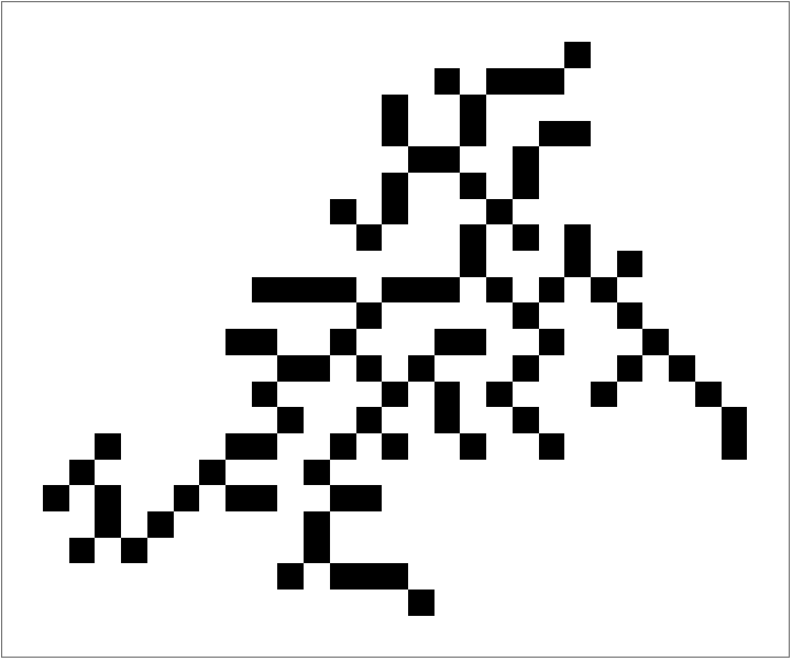
An Aggregation System describes the growth of clusters that follows a rule of aggregation. They can be simulated with a Cellular Automata with specific rules of growing. An example of this is the Eden growth model described in 1961 by Murray Eden. The idea of this model is to build up a cluster of black cells by adding just one new cell at each step . The position of this cell is chosen entirely at random, with the only constraint being that it should be adjacent to an existing cell in the cluster. However, the growing process could be more general and be described as follows: it occurs when a new black cell is added at each step and this happens in a position chosen at random among all the positions that have a certain number of black cells in its neighborhood.
The onePathSA function allows update one time step of a random CellularAutomaton. It is possible to use the whole set or rules of CellularAutomaton build-in function. To get a path of the system for thousands of time steps it should be used Nest or NestList.
onePathCA[rule_,iniCondi_]:=Module[{previousSatateAndPossibilities=({#1,Thread[Position[#2-#1,1]->1]}&@@CellularAutomaton[rule,{iniCondi,0},1(*steps*)])},NumericArray@ReplacePart[previousSatateAndPossibilities[[1]],previousSatateAndPossibilities[[2]]//RandomChoice]];(*****************************************)rule=<|"GrowthCases"->{1},"Dimension"->2,"Neighborhood"->"Moore"|>;init={{1}};states=NestList[onePathCA[rule,#]&,init,1000];systemAggregationExample=ArrayPlot/@states;ListAnimate[systemAggregationExample]
Out[]=
Here it is used the onePathCA function to get 4 images of the system each one after ten thousands steps. It means the last one is the update 40 000
figure1=Nest[onePathCA[rule,#]&,init,10000];ArrayPlot[figure1]
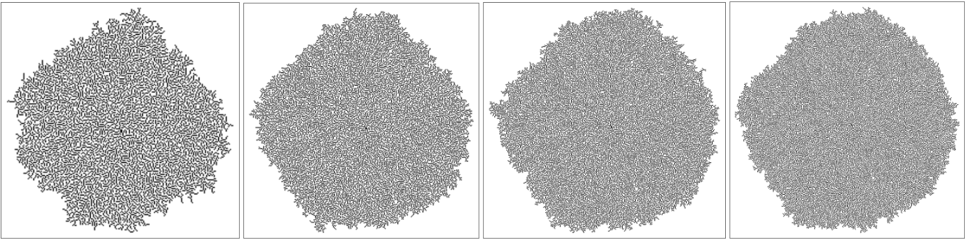
The randomness of this system is explicitly inserted from outside at each step in the evolution of the system. Due to this randomness the initial sates of the system are irregular and discontinuous but after many time steps it appears that continuous patterns of growth emerge. In this way the system aggregation in an example of a systems based on discrete components in which randomness at a microscopic level also leads to continuous behavior on a large scale. It happens because when randomness is present, such microscopic details often get averaged out, so that in the end no trace of discreteness is left, and the results appear to be smooth and continuous.
It is important to note that given an initial configuration and set of rules, the system could evolve through a finite number of new configurations to a fixed configuration in which the rules no longer apply. Or the system could grows indefinitely and form a continuous pattern as previously mentioned.
Multiway System of a System Aggregation
Multiway System of a System Aggregation
The update of a system aggregation in each time step represents one possible state from a set of possible states. It means that in each time step there are many possibilities to put a new black cell. And one realization of the system is only one path from a set of possible paths. The whole set of possible paths can be represented in a multiway system. And it could be explored the structural properties of the multiway graph to get insights into the growing pattern given a rule and initial condition.
To update the Multiway System and get the new possible states in each time steps it is used the next set of functions. The function newPossibilitiesSA gives the new possible states from one previous state. The function edgesAndNewPosibilitiesBystate built the edges list of the MultiWay Graph. The function edgesAndNewPosibilitiesByAllstates maps the previous functions in the whole set of previous states and it gets the whole set of new edges, it save them in a global variable (graph) and return the new states. The function iterationAllNewSates deletes from the new states those who are duplicates and return the new states to be updated. To update the system for several steps it should be used Nest built-in function and to display the graph it should be used showGraph function. When the graph is big it is better to used Graph or GraphPlot build-in functions.
(******************Configuration************)rule=<|"GrowthCases"->{1},"Dimension"->2,"Neighborhood"->"Moore"|>;init={{1}};(***********TogettheMultiWaySystem****)newPossibilitiesSA[rule_,iniCondi_]:=Module[{previousSatateAndPossibilities=({#1,Thread[Position[#2-#1,1]->1]}&@@CellularAutomaton[rule,{iniCondi,0},1(*steps*)])},Map[SparseArray@ReplacePart[previousSatateAndPossibilities[[1]],#]&,previousSatateAndPossibilities[[2]]]]edgesAndNewPosibilitiesBystate[state_,rule_]:=Thread[Hold[state]->newPossibilitiesSA[rule,state]]edgesAndNewPosibilitiesByAllstates[states_,rule_]:=Module[{edges},edges=ParallelMap[edgesAndNewPosibilitiesBystate[#,rule]&,states,Method"CoarsestGrained"];graph["Insert",edges];edges[[All,All,2]]]iterationAllNewSates[state_,rule_]:=DeleteDuplicates[Flatten[edgesAndNewPosibilitiesByAllstates[state,rule],1]](************Toplot*************************)showGraph[g_]:=Graph[g,VertexShape((#->ArrayPlot[#,ImageSize15])&/@VertexList[g]),GraphLayout"LayeredDigraphEmbedding",ImageSizeFull,EdgeStyleOpacity[0.4,Red]];
As an example of the Multiway System of a System Aggregation it is used the set of functions to update the system from one initial black cell to the addition of a second one.
graph=CreateDataStructure["OrderedHashSet"];Nest[iterationAllNewSates[#,rule]&,{init},1];showGraph[ReleaseHold[Flatten[(#//Normal)]]]&@(Normal[graph])

Each one of the previous states is updated to get the next set of new possible state of the system.
graph=CreateDataStructure["OrderedHashSet"];Nest[iterationAllNewSates[#,rule]&,{init},2];showGraph[ReleaseHold[Flatten[(#//Normal)]]]&@(Normal[graph])
Out[]=

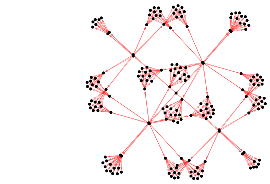
In a next iteration, the system becomes bigger. This is a example of a System Aggregation that grow exponentially.
graph=CreateDataStructure["OrderedHashSet"];Nest[iterationAllNewSates[#,rule]&,{init},3];Graph[ReleaseHold[Flatten[(#//Normal)]],ImageSizeMedium,EdgeStyleOpacity[0.4,Red],VertexStyleBlack]&@(Normal[graph])
Objective
Objective
Here it will be explored the structural properties of the Multiway System of a System Aggregation. The structural properties to evaluate are the number of new states in each time step, the vertex degree of input edges in each time step and in the whole system, the vertex degree of output edges in each time step and in the whole system, and the number of time steps that happen before the system stop its growth. These will be evaluated for a set of rules and random initial conditions.
Application
Application
This is an approximation to the study of the asymmetric tumor growth in a heterogeneous environment where there are spatial and nutritional limitations in such way that it is not possible to grow continuously in space
Experiments description
Experiments description
Rules
Rules
With the set of functions in this project it is possible to simulate whatever rule of the CellularAutomaton Built-in function. Specifically, for a System Aggregation it is used the keys “GrowthCases”, “Dimensions”, and “Neighborhood” to specify the rule as an Association. And to specify other rules of aggregation it was build a set of functions. The rules are described in the next table and some of them are plotted. Additionally, the whole set of rules are applied in two dimensions and in a Moore neighborhood
Out[]=
N° | Rule expression | Description |
1 | GrowthCases{3},Dimension2,NeighborhoodMoore | Exaclty 3 neighbors in wathever position |
2 | GrowthCases{4},Dimension2,NeighborhoodMoore | Exactly 4 neighbors in wathever position |
3 | r3[{{a_,b_,c_},{d_,i_,f_},{g_,j_,l_}}]:=If[Total[{a,b,c,d,i,f,g,j,l}]==3&&MemberQ[{{a,b,c},{b,c,f},{c,f,l},{f,l,j},{l,j,g},{j,g,d},{g,d,a},{d,a,b}},{1,1,1}],1,i] | Exaclty 3 neighbors in consecutive position |
4 | r4[{{a_,b_,c_},{d_,i_,f_},{g_,j_,l_}}]:=If[Total[{a,b,c,d,i,f,g,j,l}]==4&&MemberQ[{{a,b,c,f},{b,c,f,l},{c,f,l,j},{f,l,j,g},{l,j,g,d},{j,g,d,a},{g,d,a,b},{d,a,b,c}},{1,1,1,1}],1,i] | Exaclty 4 neighbors in consecutive position |
5 | r3[{{a_,b_,c_},{d_,i_,f_},{g_,j_,l_}}]:=If[MemberQ[{{a,b,c},{b,c,f},{c,f,l},{f,l,j},{l,j,g},{j,g,d},{g,d,a},{d,a,b}},{1,1,1}],1,i] | Minimum 3 neighbors in consecutive position |
6 | r4[{{a_,b_,c_},{d_,i_,f_},{g_,j_,l_}}]:=If[MemberQ[{{a,b,c,f},{b,c,f,l},{c,f,l,j},{f,l,j,g},{l,j,g,d},{j,g,d,a},{g,d,a,b},{d,a,b,c}},{1,1,1,1}],1,i] | Minimum 4 neighbors in consecutive position |
This is for a graphic representation of rule 1. Rule 2 is almost the same but with more neighbors
This is for a graphic representation of rule 3. Rule 4 is almost the same but with more neighbors
This is for a graphic representation of rule 5. Rule 6 is almost the same but with more neighbors. For these are required a consecutive number of black neighbors cells and it could be other neighbors in whatever position.
Initial Conditions
Initial Conditions
The simulations were performed with a random set of initial conditions in which the probability to have a black cell (wBlack) was 0.3 or 0.7.
This is a graphic representation of initial conditions.
Simulations
Simulations
For those System Aggregations with small and finite growth, it was used the set of functions previously described for the Multiway System of a System Aggregation. However, it was taken off the option Parallelize from edgesAndNewPosibilitiesByAllstates. For those System Aggregation with exponential and indefinite growth, it was used the set of functions previously described for the Multiway System without any modification.
Analysis
Analysis
To analyze the structural properties of the Multiway System and its graph it was made the next plots:
The graphList contains all the graphs of each simulation. Each graph contains all the information necessary to analyze the system. The first thing is to order the edges of each graph from the graphList. In this way it is possible to get orderly the new edges and states in each time step for each graphs in graphList.
Then it is measured the new states in each time steps for each graph and it is plotted the Mean of new states in each time step for all graphs.
Then it is measured the Convergence Level in time as the Mean of the vertex degree of input edges in each time step for all graphs.
Then it is measured the Divergence Level in time as the Mean of the vertex degree of output edges in each time step for all graphs.
Then it is plotted the number of time steps that happen before the system stop its growth
For small graphs it used this code which puts the plot of the states in each vertex
For big graphs it used this code which does not puts the plot of the states in each vertex
Then it is measured the Convergence Level for the whole systems. It means for the whole graph of each graphs in graphList
Then it is measured the Divergence Level for the whole systems. It means for the whole graph of each graphs in graphList
Results
Results
It was made a set of simulations that are summary in the next table:
The plots of the number of possible states in each time step show that for rules with less constraint (i.e. rules 1, 5, and 3) the growth is exponential. Rule 5 has more similar to rule 1 in its effect on growth than rule 3. The rules with higher constraints (i.e. rules 6, 4, and 2) drive a small growth and early stop in growing. The effect of the initial conditions is more evident in the rules with less constraint and the growth clearly increases when with the increase of black cells at the start.
Here it is uploaded the plots of the Number of possible states in each time step
While the number of new states in time differs in orders of magnitude between rules, this does not happen with the level of convergence in time. The convergence level is low and it increases slowly in time. And in general, it looks very similar between rules and initial conditions. According to these plots. It appears that the growing systems do not converge a lot.
Here it is uploaded the plots of the Convergence level in each time step
Although the divergence as the convergence does not differ in orders of magnitude it is known that these little differences between rules drive big differences in a system that could grow exponentially. For the rules with the lowest constraints, the divergence increases slowly but it is necessary to make new simulations to see the long-time behaviour. As expected, the divergence is lowest at the end of the growth for rules with higher constraints.
Here it is uploaded the plots of the Divergence level in each time step
For the rule with lest constraint (i.e rule 1) the growth happens in almost all the replicates (i.e.% occurrence 0.8-1) and for the whole time of the simulation. For rules 3 and 5, the growth in the whole time of simulation only occurs for some replicates (i.e.% occurrence 0.4, 0.6, and 0.7). For the rules with higher constraints, the percentage of occurrence is lower and in any case, they always stop growing before the last time update.
Here it is uploaded the plots of the Number of steps until stop growing. Which also show the percentage of occurrence (% occurrence) between the replicates.
With these plots of the convergence level for the whole Multiway graph, it is possible to see that the convergence could be more different between rules than previously seen. It means that the temporal mean of the convergence represented in the previous temporal plot is not a good approximation to this variable. And it also means that the convergence level is bigger for the rules with lower constraints.
Here it is uploaded the plots of the Convergence level for the whole graph
According to these plots the divergence level represented in the previous temporal plots is a good approximation for the rules with lower constraints but not for those with higher constraints. And also as was previously mentioned the first ones diverge more than the second ones.
Here it is uploaded the plots of the Convergence level for the whole graph
Finally, the next table shows some of the multiway systems that are getting for each rule. For those rules which drive a big growth (i.e. rule1, rule4, and rule 5) the system is only updated 5 times and some possible path are shown.
Here it is imported some of the multiway systems with the plot of each state as a vertex
Concluding remarks
Concluding remarks
■
Here it was explored two groups of rules with low constraints (i.e. 1,3,5) and high constraints (i.e. 2,4,6). The first one represents rules that drive exponential growth, the growth could occur indefinitely and from this will probably emerge a continuous pattern. The second one is representative of rules that drives small growth with an early stop in growing, and the system has irregular patterns. These groups could represent a threshold to grow and no-grow, respectively. Therefore, in the future study of the long-time behavior of these systems, it will be most important to focus on the first group or to make rules as combinations of both groups.
■
For those systems that grow exponentially, it appears that the divergence level has a very different behavior from the convergence level. The first one is bigger than the last one as could be expected. However, there are interesting events of high convergence in these systems that should be better studied in the long-time behavior. And it is also important to explore the rate of change of these measures.
■
The tumor growth starts when a certain microenvironment takes place in tissue and it drives the apparition of the carcinogenic cell. This could happen in different places and in this way random initial conditions could represent in a better way the initial states of the tumor growth. Additionally, it is still necessary to reflect more on how the rules of aggregation could explain or could be related to the mechanism behind tumor growth.
■
Because the divergence and convergence levels have particular behavior and they are tightly associated with the possible random changes the system can have, it is important to reflect more on how these measures could explain the next statement: : “... As a rough guide, it seems that continuous patterns of growth are possible only when the rate at which small - scale random changes occur is substantially greater than the overall rate of growth. In general the point is that continuous behavior can arise in systems with discrete components only when there are features that evolve slowly relative to the rate of small-scale random changes..” (NKS book)
■
Finally, it was built an efficient and simple function to track the growth of a System Aggregation. And the set of functions to get the Multiway System of a System Aggregation work pretty well for rules that drive small growth. However, for rules that drive exponential growth, it is necessary to improve the performance of the functions in such a way that they spend less memory. One possible idea is to split the possible new states into groups that are evaluated sequentially but evaluate each one of them in parallel. In this way, it is reduced the amount of memory required to process the states in each iteration.
Keywords
Keywords
◼
System Aggregation
◼
Multiway System
◼
Tumor growth
Acknowledgment
Acknowledgment
I would like to express my special thanks of gratitude to Stephen Wolfram who gave me the golden opportunity to do this wonderful Summer School and project. My special thanks to my mentor Jesse Galef for the constant support. Also thanks to Robert Nachbar and Xerxes Arsiwalla for their advice. I also wanted to thanks the TAs team in special to Jesse Friedman, Daniel Sanchez, and Silvia Hao. And last but not least thanks to Erin Cherry, Mads Bahrami, and Danielle Rommel.
References
References