Exploring the gender gap in the labor market: an evolutionary approach
by Zazueta Jorge, Accinelli Elvio
by Zazueta Jorge, Accinelli Elvio
Article Abstract
Article Abstract
We develop a simple mathematical model describing the dynamics of the gender gap in a labor market niche and study the effects of bias, market size, and market dynamism in the evolution of the system. A high-level characterization of the system is suggested by studying a large sample of the parameter space, and specific cases of interest to policy-making are explored. This paper aims to present a model that serves as a tool to examine the implications of policy decisions and explore some of these implications to shed some light on future policy-making intended to address the gender gap.
The Model
The Model
We assume a labor market with a given carrying K capacity that recruits talent from a pool of male and female applicants with uniform sex distribution and identical talent. The labor market is integrated by males and females with fixed preferences and biases towards recruiting their own and opposite sex, determine the recruiting dynamics. Members of the labor market niche also leave due to a variety of reasons such as promotion, retirement or even death in proportion to a market dynamism constant, specific to each sex. This can be represented by the following dynamical system:
y
x
x
t
λ
wm
λ
ww
r
x
y
t
λ
mm
λ
mw
r
y
Where is the market carrying capacity, represents the strength of support of sex for recruiting sex , and ≤ 1 is the proportion of sex leaving the niche. We can simplify the system by selecting the appropriate units so that and by choosing the strength constants such that 0 ⩽≤1 and + = 1 for all in . This way we can interpret as a proportions and reduce the number of parameters from by 3. Letting = and we can rewrite the system as:
K
λ
ij
i
j
0≤
r
i
i
K=1
λ
ij
λ
ik
λ
jk
i,jandk
{w,m}
λ
ij
α
λ
ww
β=
λ
mm
x
t
r
x
y
t
r
y
Note that our definition of the support and bias from one sex to the other need to be symmetrical and complete. That is, if women support women by α, the necessarily support men by . Men behave similarly.
αandβ
(1-α)
General Model Dynamics
General Model Dynamics
The system has up to three equilibrium points at the intersection of the to hyperbolas defined by the equations:
F=(1-x-y)(y(1-β)+xα)-x=0G=(1-x-y)(yβ+x(1-α))-y=0
r
x
r
y
Notice that only two of the three equilibria lie within our domain of interest: (1) the unstable trivial equilibrium and the attractor in the region . For the rest of this paper, we will only consider equilibria within this region.
(0,0)
[0,1]x[0,1]
In[]:=
{xstart,xend}={-4,1};{ystart,yend}={-1,4};sol1=ParametricNDSolve[{[t](a*x[t]+(1-b)*y[t])*(1-x[t]-y[t])-r1x[t],[t]((1-a)*x[t]+b*y[t])*(1-x[t]-y[t])-r2y[t],x[0]0.01,y[0]0.015},{x,y},{t,100},{a,b,r1,r2}];Manipulate[GraphicsRow[{Show[{ContourPlot[{(ax+(1-b)y)(1-x-y)r1x,((1-a)x+by)(1-x-y)r2y},{x,xstart,xend},{y,ystart,yend},ContourStyle{Thickness[.012]},PlotLabel"Direction Field and Fixed Points",FrameLabel{Women,Men},ImageSize267],StreamPlot[{(ax+(1-b)y)(1-x-y)-r1x,((1-a)x+by)(1-x-y)-r2y},{x,xstart,xend},{y,ystart,yend},StreamStyleGray],ListPlot[{x,y}/.NSolve[{(ax+(1-b)y)(1-x-y)r1x,((1-a)x+by)(1-x-y)r2y},{x,y}],PlotStyle{Gray,PointSize[0.035]}]}],Plot[{x[a,b,r1,r2][t]/.sol1,y[a,b,r1,r2][t]/.sol1},{t,0,Time},Filling{1{2}},PlotLabel"Women and Men Labour Market Dynamics",AxesLabel{"Time","Employed"},PlotLabels{"Women","Men"},ImageSize300]}],{{a,0.7},0,1,Appearance"Labeled"},{{b,0.65},0,1,Appearance"Labeled"},{{r1,0.5},0,1,Appearance"Labeled"},{{r2,0.4},0,1,Appearance"Labeled"},{{Time,30},0,100,Appearance"Labeled"},SaveDefinitionsTrue]
′
x
′
y
Out[]=


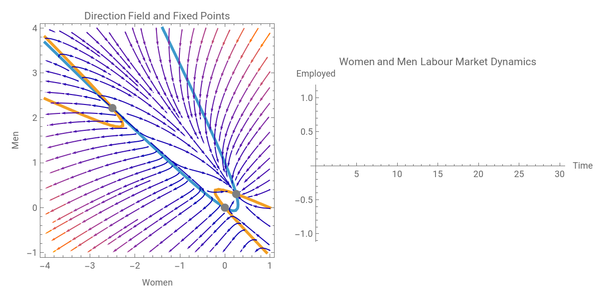
On the right side of the panel we can see how the gap between sexes widens until the market is saturated and stabilizes with a mix that, in this particular case, favors men. Our main question is how can gender equality be achieved starting from a scenario where males represent the majority of the population. The rest of the paper explores this question through a handful of scenarios.
The Naive Model
The Naive Model
We start by considering a setting without selection biases and every employee is hired based solely on its professional merits. Furhtermore, employees do not leave their jobs during the period under study. Our system of equations will be reduced to:
In[]:=
Dt[x,{t}]=(-x-y+1)(x+y)Dt[y,{t}]=(-x-y+1)(x+y)
1
2
1
2
The solutions for this simplified system can be found in closed form:
In[]:=
solNaive=DSolve[{x'[t](1/2)(1-x[t]-y[t])(x[t]+y[t]),y'[t](1/2)(1-x[t]-y[t])(x[t]+y[t])},(*x[0]0.015,y[0]0.015},*){x,y},t]
Out[]=
yFunction{t},+--,xFunction{t},--
1
t
t
1
2
2
1
2(+)
t
2
2
t
t
1
2
2
1
2(+)
t
2
2
In[]:=
FullSimplify[%]
Out[]=
yFunction{t},+--,xFunction{t},--
1
t
t
1
2
2
1
2(+)
t
2
2
t
t
1
2
2
1
2(+)
t
2
2
Which implies that . That is: a perfectly unbiased hiring environment, in the absence of market dynamism, preserves the current gender gap. Under the assumptions of our model, gap dynamics respond both to bias and market dynamism sometimes in not immediately obvious ways. We now introduce bias back into the system, while keeping market dynamism out.
y-x=
c
1
Introducing Bias without Market Dynamism
Introducing Bias without Market Dynamism
Reintroducing our bias parameters, our system becomes:
αandβ
In[]:=
x
t
y
t
Fixed points are the origin . We restrict our attention to the region [0,1]x [0,1].
(0,0)andthoseontheline{(x,y)|x+y=1}
In[]:=
solNoDyn=ParametricNDSolve[{x'[t](a*x[t]+(1-b)*y[t])*(1-x[t]-y[t]),y'[t]((1-a)*x[t]+b*y[t])*(1-x[t]-y[t]),x[0]==0.1,y[0]==0.15},{x,y},{t,100},{a,b}];Manipulate[GraphicsRow[{Show[{StreamPlot[{(ax+(1-b)y)(1-x-y),((1-a)x+by)(1-x-y)},{x,0,1},{y,0,1},ImageSize267],ContourPlot[{(ax+(1-b)y)(1-x-y)0,((1-a)x+by)(1-x-y)0},{x,0,1},{y,0,1}]},PlotLabel"Direction Field and Fixed Points",FrameLabel{"Women","Men"}],Plot[{x[a,b][t]/.solNoDyn,y[a,b][t]/.solNoDyn},{t,0,10},Filling{1{2}},PlotLabel"Women and Men Labor Market Behaviour",AxesLabel{"Time","Employed"},PlotLabels{"Women","Men"},ImageSize295]}],{{a,0.75},0,1,Appearance"Labeled"},{{b,0.6},0,1,Appearance"Labeled"},SaveDefinitionsTrue]
Out[]=
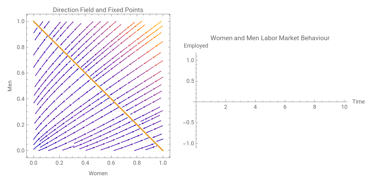
As the figure suggests, for some values of , the number of employed women can reach and surpass the number of men even when the initial conditions where unfavorable for women. ---While our focus will be on the region below the fixed points line, the upper side can be interpreted as an overcrowded market that naturally corrects itself by evolving towards the fixed line---That is, we are interested in parameter combinations such that the initially lower women curve, reaches or crosses the male curve. In principle, we should strive to identify parameters that result in an equality equilibrium, but this approach is impractical from a policy-making point of view where it would be more efficient to identify reasonable policies that increase the job generation speed for women and readjust once equity is achieved. To simplify the analysis, we define the gender gap
αandβ
γ(α,β,,)=y(α,β,,)-x(α,β,,)
x
0
y
0
x
0
y
0
x
0
y
0
Conclusions
Conclusions
◼
A perfectly unbiased hiring environment, in the absence of market dynamism, preserves the existing gender gap.
◼
Given equal initial conditions, the requisite change in α increases in the opposite direction of market capacity, suggesting that a healthy, growing labor market is more conducive to gender equality under the same preference and bias assumptions. As the market saturates, an equilibrium is reached and no change in preferences, either natural or induced will have an effect on the population proportion. As these proportions become less favorable, the policy range might shrink out of scope even with a relatively large market.