Abstract: The construction of multi-soliton solutions for the nonlinear Schrödinger equation, also known as the Gross–Pitaevskii equation, serves as a foundational exploration into the nature of localized wave phenomena. Utilizing the Hirota bilinear method, this work systematically extends the framework from single wave packets to complex systems involving up to three interacting solitons. This formal structure provides a rigorous basis for representing the interference patterns and non-linear couplings inherent in integrable systems.
Central to this investigation is the integration of these mathematical solutions with the causal interpretation of quantum mechanics, called the de Broglie-Bohm pilot-wave theory or Bohmian mechanics. This study addresses the enduring wave-particle duality by examining the evolution of wave density and velocity fields, where the quantum potential serves as the fundamental mechanism orchestrating particle trajectories during elastic collisions. Rather than treating waves and particles as inherently separate entities, this Bohmian approach suggests a compelling ontological pattern: a non-linear field may exhibit particle-like properties—such as finite, localized energy, structural stability through collisions, and specific interaction signatures—without being the particle itself. Instead, the field acts as a pilot structure, guiding discrete points through space-time while maintaining the coherence of the system.
The analysis highlights the characteristic phase shifts and the systematic redistribution of energy and density observed during multi-soliton interactions. Furthermore, the discussion touches upon highly speculative implications for nuclear physics. By modeling coherent structures as pilot-wave entities, this perspective invites a re-evaluation of the relationship between field-theoretic descriptions and localized matter, potentially offering new avenues for understanding collective phenomena and the emergence of structural stability in physical systems.
Central to this investigation is the integration of these mathematical solutions with the causal interpretation of quantum mechanics, called the de Broglie-Bohm pilot-wave theory or Bohmian mechanics. This study addresses the enduring wave-particle duality by examining the evolution of wave density and velocity fields, where the quantum potential serves as the fundamental mechanism orchestrating particle trajectories during elastic collisions. Rather than treating waves and particles as inherently separate entities, this Bohmian approach suggests a compelling ontological pattern: a non-linear field may exhibit particle-like properties—such as finite, localized energy, structural stability through collisions, and specific interaction signatures—without being the particle itself. Instead, the field acts as a pilot structure, guiding discrete points through space-time while maintaining the coherence of the system.
The analysis highlights the characteristic phase shifts and the systematic redistribution of energy and density observed during multi-soliton interactions. Furthermore, the discussion touches upon highly speculative implications for nuclear physics. By modeling coherent structures as pilot-wave entities, this perspective invites a re-evaluation of the relationship between field-theoretic descriptions and localized matter, potentially offering new avenues for understanding collective phenomena and the emergence of structural stability in physical systems.
Full list of posts: https://community.wolfram.com/web/kvbloh/
Note: see the detailed introduction to the de Broglie Bohm theory with Mathematica here:
Introduction to the Bohm-De Broglie Theory: The Causal Interpretation of the Quantum Theory
Nonlinear Schrödinger Equation (NLS) in the Causal Interpretation (de Broglie Bohm theory)
Introduction to the Hirota direct method with the trajectory approach to solitons
Note: see the detailed introduction to the de Broglie Bohm theory with Mathematica here:
Introduction to the Bohm-De Broglie Theory: The Causal Interpretation of the Quantum Theory
Nonlinear Schrödinger Equation (NLS) in the Causal Interpretation (de Broglie Bohm theory)
Introduction to the Hirota direct method with the trajectory approach to solitons
0. Introduction
0. Introduction
Sometimes it is necessary to end a Wolfram Language kernel session or to clear all values, definitions, attributes, defaults, options and messages for the symbols.
In[]:=
Quit[]
In[]:=
ClearAll["Global`*"]
Use the following command, if you need to save/export graphs created by Mathematica into the current notebook directory:
In[]:=
SetDirectory[NotebookDirectory[]]
Out[]=
I:\Mathematica Notebooks
To make the equations more readable, the standard form of partial derivatives is used. The definition is taken from the Wolfram blog.
In[]:=
pdConv[f_]:=TraditionalForm[f/.Derivative[inds__][g_][vars__]:>Apply[Defer[D[g[vars],##]]&,Transpose[{{vars},{inds}}]/.{{var_,0}:>Sequence[],{var_,1}:>{var}}]]
Cells that contain ‘dynamic content’ often lead to a system message. As a result, it is sometimes necessary to switch off dynamic evaluation for certain calculations.
PaletteNotebook@Column[{Button["Dynamic off",SetOptions[NotebookSelection[],DynamicUpdating->False]],Button["Dynamic on",SetOptions[NotebookSelection[],DynamicUpdating->True]]}]
In[]:=
SetOptions[$FrontEnd,"DynamicEvaluationTimeout"->30]
Feel free to use, reproduce, and modify this code in its entirety or in part of it. A further note: Some descriptions might be formulated too simply and could possibly require a more detailed explanation.
WARNING: These notes are incomplete and may contain errors in the implementation of the code and in the implementation of the equations. Although every step in the derivation of the non-linear Schrödinger equation has been meticulously checked, potential errors may still exist. The essay has been written to the best of my knowledge and with great care. Every equation has been checked. It cannot be ruled out that errors may still exist. Some of the formulations are not introduced with mathematical precision and may contain linguistic inaccuracies. To simplify calculations, SI units are not used throughout this work. The author hopes, that readability is not significantly affected by this. The essay has not undergone a detailed peer review. Attention was paid to the clarity and comprehensibility of the equations. Therefore, many equations were not combined into a single expression. This sometimes results in less than optimal computational efficiency. I applied parallelization of the computational steps only in areas where a significant increase in processing speed could be achieved. They rather serve didactic purposes and aim to contribute to an understanding of handling mathematics with Mathematica. Similarly, I have not indicated quotes from my own works. To the best of my knowledge, I have listed all individuals from whom I have adopted parts of the programs. If I have overlooked people who have contributed to Bohm’s theory or to the algorithms used, this is solely my responsibility.
A note to the reader: Some of the equations and algebraic rearrangements are admittedly rather large, which can make for strenuous reading at times. The author hopes that this step-by-step approach nevertheless helps the reader follow every derivation in detail.
WARNING: These notes are incomplete and may contain errors in the implementation of the code and in the implementation of the equations. Although every step in the derivation of the non-linear Schrödinger equation has been meticulously checked, potential errors may still exist. The essay has been written to the best of my knowledge and with great care. Every equation has been checked. It cannot be ruled out that errors may still exist. Some of the formulations are not introduced with mathematical precision and may contain linguistic inaccuracies. To simplify calculations, SI units are not used throughout this work. The author hopes, that readability is not significantly affected by this. The essay has not undergone a detailed peer review. Attention was paid to the clarity and comprehensibility of the equations. Therefore, many equations were not combined into a single expression. This sometimes results in less than optimal computational efficiency. I applied parallelization of the computational steps only in areas where a significant increase in processing speed could be achieved. They rather serve didactic purposes and aim to contribute to an understanding of handling mathematics with Mathematica. Similarly, I have not indicated quotes from my own works. To the best of my knowledge, I have listed all individuals from whom I have adopted parts of the programs. If I have overlooked people who have contributed to Bohm’s theory or to the algorithms used, this is solely my responsibility.
A note to the reader: Some of the equations and algebraic rearrangements are admittedly rather large, which can make for strenuous reading at times. The author hopes that this step-by-step approach nevertheless helps the reader follow every derivation in detail.
CAUTION! Enter parameters as rational numbers if possible, so that numerics are as accurate as possible.






Figure
0
. Vladimir Zakharov (1939-2023), Alexey Shabat (1937-2020), Ryōgo Hirota (1932–2015), Ludwig Dmitrijewitsch Faddeev(1934-2017) , Leon Armenowitsch Takhtajan (1950), Eugene Paul Gross (1926 – 1991) and Lev Pitaevskii (1933-2022) (images from [Wikipedia and Alchetron]). 

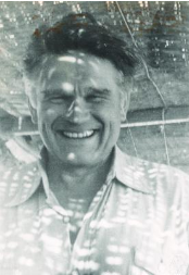
Figure 1. Chris Eilbeck, Alwyn C. Scott, and Martin Kruskal (left to right) waiting for a Scott Russell soliton water wave (1995) (image from Journal of Biological Physics [28] and from from the web: John Scott Russell's Soliton Wave Re-created).
1. Introduction
1. Introduction
Solitons are localized wave structures that arise in nonlinear dispersive systems and exhibit remarkable stability properties ([1]-[11]). Unlike linear wave packets, which typically spread over time due to dispersion, solitons preserve their shape during propagation. This behavior is a purely nonlinear phenomenon resulting from an exact balance between dispersion and nonlinearity. Moreover, solitons are characterized by finite energy, which can often be expressed in terms of a conserved Hamiltonian of the underlying system. They also exhibit particle-like properties, such as elastic interactions with other solitons (for examples: [5], [6], [9], [11].Historically, the physical phenomenon at the origin of this theory was first observed in 1834 by the Scottish engineer John Scott Russell [29], who tracked and described a form-stable, solitary water wave traveling along a canal. In the 1960s, the US mathematician Martin Kruskal provided the rigorous mathematical foundation for this phenomenon, proving that these waves retain their shape even after collisions, and coined the modern term “soliton” to reflect their particle-like behavior [11]. The US physicist Alwyn C. Scott subsequently built upon these theories, playing a pivotal role in popularizing the concept and expanding its application to other disciplines, including biology and optics [28]. Completing the group, the British mathematician J. Chris Eilbeck, a close collaborator of Scott, further advanced the field and organized the 1995 historical re-enactment of the canal experiment, generating the very wave that Kruskal and Scott were waiting to witness in the photograph (photograph taken from [28]) .One of the most important equations supporting soliton solutions is the nonlinear Schrödinger equation (NLS) often called Gross–Pitaevskii equation [20], which appears in various physical contexts such as nonlinear optics [8], fluid dynamics ([9], [6], [10]), and plasma physics [1] and possesses rich structures, for example [10]: . The NLS equation is a nonlinear partial differential equation [27] that describes the evolution of a complex-valued wavefunction.In the linear limit with the NLS goes into the linear Schrödinger equation for a wave function of a free one-dimensional particle with mass with a general solution with ,∈C.
i++2|uu0
u
t
u
xx
2
|
2|uu0
2
|
m
1
2
u(x,t)
γ
0
ix-t
λ
0
2
λ
0
e
λ
0
γ
0
In[]:=
SE[u_]:=ID[u,t]+D[u,{x,2}];u=γ0Exp[I(λ0x-λ0^2t)];result=Simplify[SE[u]];Print["The identity holds: ",Style[Simplify[result==0],Black,Bold]];
The identity holds: True
In addition to quantum mechanics and optics, the Nonlinear Schrödinger equation serves as a fundamental model in hydrodynamics, particularly for the propagation of deep-water waves [9]. In this context, the NLS equation describes the evolution of a modulated wave train on the ocean surface, balancing dispersive effects with convective nonlinearities. This mathematical framework is of crucial importance in physical oceanography, as it successfully models the formation and stability of envelope solitons, as well as the emergence of extreme, spontaneous rogue waves. Interpreting these hydrodynamic systems through a Bohmian lens offers an insightful causal map, where the computed trajectories translate directly into the actual paths of fluid particles or the localized transport of kinetic energy beneath the surface of the undulating water column.The Hirota bilinear method has been applied successfully to many soliton equations, including the construction of resonance soliton solutions of the NLS equation by Pashaev and Lee [5]. The Bohmian perspective on these resonance solitons was already addressed by the author in an earlier Wolfram Demonstration (see Appendix), highlighting the method’s ability to bridge algebraic solution techniques and physical particle trajectories.The Hirota bilinear method transforms a nonlinear PDE into a set of bilinear equations via the substitution . These equations are bilinear [22] (the Wikipedia entry on bilinear forms is primarily algebraic) in and and their derivatives, and can be solved systematically using exponential series, leading to compact determinant representations for multi-soliton solutions.In the context of the nonlinear Schrödinger (NLS) equation solved via the Hirota bilinear method, the physical characteristics of each soliton are entirely determined by its complex wavenumber, typically denoted as +i. Unlike the Korteweg-de Vries (KdV) equation, where a soliton’s amplitude fundamentally dictates its speed, the NLS equation decouples these dynamical properties. Specifically, the real part of the wavenumber, , governs the peak amplitude and the spatial width, or localization, of the wave envelope. In contrast, the imaginary part, , independently dictates the propagation velocity and phase evolution of the soliton. Consequently, within the NLS framework, it is entirely possible for a soliton to possess a highly concentrated energy density with a large amplitude while remaining strictly stationary, or conversely, to exhibit a very small amplitude while propagating rapidly through the medium. Throughout this work, the complex wavenumber is denoted as +ik, where alternative subscript notations for the imaginary part, such as , may be used interchangeably depending on the context.
ug/f
g
f
k
j
η
j
ξ
j
η
j
ξ
j
k
j
C
j
k
Cj
2. Derivation of the Bilinear Form of the NLS using the Hirota Method
2. Derivation of the Bilinear Form of the NLS using the Hirota Method
The nonlinear Schrödinger equation (NLS) with being complex can be transformed into a bilinear form [22] using the substitution where is real-valued and is complex-valued . This leads to the bilinear system ([3], [4]).where and denote Hirota’s bilinear differential operators, defined by a·ba(x)b()x,a·ba(t)b()t.Expanding the Hirota operators yields(a·b)
ba.(a·b)
ba.The two bilinear equations should be viewed as a sufficient condition for solving the nonlinear Schrödinger equation. If both bilinear equations hold, then the Hirota-transformed field satisfies the NLS. The converse implication is not required for the present construction and is not addressed here. Since the goal is the explicit generation of soliton solutions, the sufficiency of the bilinear system is entirely sufficient for the purposes of this work.Examples:G·FF-G,G·FF-2+G,F·F2F-.Remark: Throughout this work, the notation denotes the complex conjugate of . In some parts of the physics literature, the alternative notation is used for the same operation. Since the symbol may denote either complex conjugation or, in other contexts, an adjoint operation, some ambiguity may arise in the literature. Symbolic computation systems such as Mathematica commonly employ the star notation. For this reason, both notations , or will be used interchangeably in the following, always referring to complex conjugation.Derivatives of : First, the required partial derivatives are calculated.First time derivativeF-G.First spatial derivativeF-G.Second spatial derivative is calculated with :-A·2F.Then, F+--GF-G.Substituting yields.Expanding:-G-2+2GFF-G-2+2G.The Nonlinear term gives:Substitution into the NLSSubstituting all terms into i++2|uu0, it follows:Multiplication by Regrouping the terms: Step 1: Time term.Step 2: Second derivatives in .-2F. Adding and subtracting the term : -2F(-2F+GF)-GF. Factoring out an in the first term in parentheses:Using the definition of the Hirota operator, it follows:Step 3: Substitution into the overall equation. Thus, the initial equation becomes:Step 4: Combining the terms. The two terms involving are: Since multiplication is commutative:This results in:Step 5: Representation via F·F. The combination is:With F·F2F- it follows:Step 6: Final form: or in linear formSplitting into two bilinear equations. And finally, the NLS equation is satisfied if the following two bilinear equations hold simultaneously:(G,F):i+G·F0,(G,F):F·F2|G2 G.The naming of the equations often follows the order of the terms in : corresponds to the first-order equation (), which yields the linear dispersion relation and determines . corresponds to the coefficient equation arising at order . Since the NLS equation features a cubic nonlinearity (), the first non-trivial interaction between solitons occurs at this third order. The notation and follows the standard Hirota perturbation expansion, where the subscripts indicate the order in the formal expansion parameter .Written out, the two equations are:This is the desired bilinear system, whose solutions generate solutions of the NLS equation through the transformation .Thus, the nonlinear equation is transformed into a system of equations that are linear (in the Hirota derivatives), which can be solved using the method of bilinear forms (e.g., by perturbation theory or direct search for soliton solutions).Conclusion:The central identity of the Hirota method states that the original NLS equation, multiplied by , is exactly equivalent towhere and are the Hirota bilinear operators defined above. Consequently, solving the two bilinear equations is sufficient to guarantee a solution of the NLS. The identityis implemented in the Mathematica code asHere corresponds to (, whereas to (F·F)-2 G, and the substitution enforces the real-valued function . The result reproduces exactly the left-hand side of the central Hirota identity.
i++2|uu0
u
t
u
xx
2
|
u(x,t)
u,
G
F
F
G
i+G·F0,F·F2 G,
D
t
2
D
x
2
D
x
G
D
x
D
t
n
D
x
n
(-)
∂
x
∂
′
x
′
x
|
′
x
m
D
t
m
(-)
∂
t
∂
′
t
′
t
|
′
t
n
D
x
n
∑
i0
n |
i |
i
(-1)
i
∂
∂
i
x
n-i
∂
∂
n-i
x
n
D
t
n
∑
i0
n |
i |
i
(-1)
i
∂
∂
i
t
n-i
∂
∂
n-i
t
D
t
G
t
F
t
2
D
x
G
xx
G
x
F
x
F
xx
2
D
x
F
xx
2
F
x
G
G
*
G
*
G
G
GC
*
G
u
u
t
G
t
F
t
2
F
u
x
G
x
F
x
2
F
AF-G
G
x
F
x
u
xx
A
x
2
F
F
x
4
F
A
x
(F-G)
G
x
F
x
x
G
xx
G
x
F
x
G
x
F
x
F
xx
G
xx
F
xx
u
xx
(F-G)-2F(F-G)
G
xx
F
xx
2
F
F
x
G
x
F
x
4
F
u
xx
G
xx
3
F
F
xx
2
F
G
x
2
F
F
x
2
F
x
4
F
G
xx
F
xx
G
x
F
x
2
F
2
F
x
3
F
uu·.
2
|
2
G
F
G
F
G
G
2
F
G
F
GG
2
|
3
F
u
t
u
xx
2
|
iF-G+F-G-2+2G+20.
G
t
F
t
2
F
G
xx
F
xx
G
x
F
x
2
F
2
F
x
3
F
GG
2
|
3
F
3
F
iF(F-G)+F(F-G-2)+2G+2GG0.
G
t
F
t
G
xx
F
xx
G
x
F
x
2
F
x
2
|
i-GF+(-GF-2F)+2G+2GG0.
G
t
2
F
F
t
G
xx
2
F
F
xx
G
x
F
x
2
F
x
2
|
i-GFiF(F-G)F·iG·F.
G
t
2
F
F
t
G
t
F
t
D
t
x
G
xx
2
F
G
x
F
x
GF
F
xx
G
xx
2
F
G
x
F
x
G
xx
2
F
G
x
F
x
F
xx
F
xx
F
...F(F-2+G)-GF.
G
xx
G
x
F
x
F
xx
F
xx
...F·G·F-GF.
2
D
x
F
xx
F·iG·F+F·G·F-GF-GF+2G+2GG0.
D
t
2
D
x
F
xx
F
xx
2
F
x
2
|
F
xx
F
xx
-GFand-GF.
F
xx
F
xx
-GF-GF-2GF.
F
xx
F
xx
F
xx
FiG·F+G·F-2GF+2G+2GG0.
D
t
2
D
x
F
xx
2
F
x
2
|
2
D
x
-2GF+2G-G2F-2.
F
xx
2
F
x
F
xx
2
F
x
2
D
x
F
xx
2
F
x
-2GF+2G-G·F·F.
F
xx
2
F
x
2
D
x
FiG·F+G·F-GF·F+2GG0,
D
t
2
D
x
2
D
x
2
|
FiG·F+G·F-GF·F-2|G0.
D
t
2
D
x
2
D
x
2
|
H
1
D
t
2
D
x
H
3
2
D
x
2
|
G
G
H
1
O()
1
ϵ
G
1
H
3
O()
3
ϵ
uu
2
|
H
1
H
3
ϵ
i(F-G)+F-2+G0,2F-2|G⟺ F-G.
G
t
F
t
G
xx
G
x
F
x
F
xx
F
xx
2
F
x
2
|
F
xx
2
F
x
2
|
uG/F
3
F
F·i+(G·F)- G·(F·F)-2G0 ,
D
t
2
D
x
2
D
x
G
D
x
D
t
i+(G·F)0 ,(F·F)2G,
D
t
2
D
x
2
D
x
G
F·i+(G·F)- G·(F·F)-2 G0
D
t
2
D
x
2
D
x
G
expr(F[x,t]*HirotaNLS1[F[x,t],G[x,t]]-G[x,t]*HirotaNLS2[F[x,t],G[x,t],Conjugate[G[x,t]]]//Expand)/.Conjugate[F[t]]->F[x,t];
x
,
HirotaNLS1
i+(G·F)
D
t
2
D
x
HirotaNLS2
2
D
x
G
Conjugate[F[x_,t_]]->F[x,t]
F
expr
Remark: The construction of multi-soliton solutions for the nonlinear Schrödinger equation serves as a foundational exploration into the nature of localized wave phenomena. Utilizing the Hirota bilinear method, this work systematically extends the framework from single wave packets to complex systems involving up to three interacting solitons. This formal structure provides a rigorous basis for representing the interference patterns and non-linear couplings inherent in integrable systems. To preserve the introductory nature of the presentation and keep the focus squarely on the physical insights, advanced algebraic structures such as determinants, Pfaffians, and Plücker relations, along with complex matrix operations, are omitted, as their inclusion would require a lengthy mathematical detour. Furthermore, the deeper algebraic foundations of the Hirota method, including determinant representations, Pfaffians, and Plücker relations, are intentionally omitted. These topics are mathematically sophisticated and often require substantial additional background. The present work therefore focuses on the direct constructive aspects of the method, illustrating that meaningful physical and mathematical insights can be obtained without mastering every advanced algebraic detail of the theory. The derivation above establishes that solving the two bilinear equations is sufficient to construct solutions of the nonlinear Schrödinger equation. Since the objective of the present work is the explicit construction of soliton solutions, no proof of the converse implication is required.
2.1 Hirota Perturbation Expansion and the One - Soliton Solution
2.1 Hirota Perturbation Expansion and the One - Soliton Solution
2.2 Transformation to the Hyperbolic Secant Form
2.2 Transformation to the Hyperbolic Secant Form
3.1 Algebraic System for the Two‑Soliton Coefficients
3.1 Algebraic System for the Two‑Soliton Coefficients
3.2 Blockwise Solution of the System of Equations
3.2 Blockwise Solution of the System of Equations
4 Hirota' s N- Soliton Solution for the Focusing NLS Equation
4 Hirota' s N- Soliton Solution for the Focusing NLS Equation
4.1 Gram Determinant and Squared Vandermonde Product
4.1 Gram Determinant and Squared Vandermonde Product
4.2 The Internal Interaction Factor A (S) and B(S)
4.2 The Internal Interaction Factor A (S) and B(S)
4.4 Explicit Example : N = 2 (Two Solitons)
4.4 Explicit Example : N = 2 (Two Solitons)
4.4 The Coefficients A(S), B(T) and C(S,T) in the Three-Soliton Solution
4.4 The Coefficients A(S), B(T) and C(S,T) in the Three-Soliton Solution
4.5 Remark on the Special Wave Number Combination
4.5 Remark on the Special Wave Number Combination
4.6 Completely worked out 2‑soliton example
4.6 Completely worked out 2‑soliton example
5 The Listing in Detail
5 The Listing in Detail
5.1 Example N=1
5.1 Example N=1
5.2 Example N=2
5.2 Example N=2
5.3 Example N=3
5.3 Example N=3
6 Introduction to Bohmian mechanics
6 Introduction to Bohmian mechanics
6.1 Phase and Amplitude of a Soliton Solution in Hirota Form
6.1 Phase and Amplitude of a Soliton Solution in Hirota Form
6.2 Energy and Hamiltonian Structure of Soliton Solutions
6.2 Energy and Hamiltonian Structure of Soliton Solutions
6.2.2 Energy of the One - Soliton Solution
6.2.2 Energy of the One - Soliton Solution
7 One-Soliton Solution with Closed-Form Density, Phase, and an Analytic Equation of Motion
7 One-Soliton Solution with Closed-Form Density, Phase, and an Analytic Equation of Motion
To visualize the dynamical evolution of the Bohmian trajectories in relation to the wave density, a specialized visualization routine is used. Similar to the peak extraction tool, this function has been adapted from a previous notebook to automate the numerical integration of the guiding equation and the subsequent graphical representation.
The graph displays the wavefunction’s density on the left, with the possible trajectories originating from different starting points in the center, and a combined view of both the wave density and trajectories on the right. The procedure myFinalPlot must be executed beforehand so that the trajectories can be used in the following code.
This video provides a dual-panel visualization of NLS solitons within the framework of Bohmian mechanics, offering a comprehensive diagnostic of the causal evolution by simultaneously displaying the wave density, the velocity field, and the quantum potential
8 Two-Soliton Solutions and Particle Trajectories
8 Two-Soliton Solutions and Particle Trajectories
The graph displays the wavefunction’s density on the left, with the possible trajectories originating from different starting points in the center, and a combined view of both the wave density and trajectories on the right.
9 Three-Soliton Solutions and Particle Trajectories
9 Three-Soliton Solutions and Particle Trajectories
The graph displays the wavefunction’s density on the left, with the possible trajectories originating from different starting points in the center, and a combined view of both the wave density and trajectories on the right.
This visualization provides a dual-panel analysis of three-soliton interactions within the framework of Bohmian mechanics, offering a comprehensive diagnostic of the causal evolution. The left panel simultaneously displays the wave density, the velocity field, the quantum potential and the discrete particle positions, while the right panel illustrates the particle trajectories superimposed on the space-time density plot. In this system, the three solitons undergo a sequence of elastic collisions. Because the NLS equation is integrable, each soliton preserves its individual identity, amplitude, and velocity following the interaction, yet the entire configuration undergoes a global transformation. During this process, the quantum potential functions as the primary driver of particle motion, continuously guiding the particles through the complex interference patterns generated by the overlapping wave packets. The solitons exhibit distinct phase shifts, and the interaction results in a systematic exchange of positions: the fastest soliton overtakes the others, while the slowest is displaced accordingly. The middle soliton serves as a stable anchor in the interaction sequence. It interacts sequentially with both the faster and the slower wave packets, effectively “passing through” the collision zone while maintaining its relative spectral characteristics. Throughout these events, the visualization reveals how energy and wave density are dynamically transferred between all three solitons (in the Bohmian view). The Bohmian particles are intricately guided by the rapidly evolving topology of the quantum potential, clearly demonstrating how the density redistribution is orchestrated during the complex transition of these three coherent structures.
10 Four - Soliton Solutions and Particle Trajectories
10 Four - Soliton Solutions and Particle Trajectories
11 Speculative Implications for Nuclear Physics
11 Speculative Implications for Nuclear Physics
Beyond the formal description of soliton dynamics, the Bohmian extension of the nonlinear Schrödinger equation suggests a broader ontological perspective: a nonlinear field may exhibit localized, particle-like properties — such as stability, energy concentration, and characteristic interaction behavior — without itself being identical to a particle in the conventional sense.
Within this framework, the wave structure functions as a guiding entity that organizes and constrains the motion of localized degrees of freedom through spacetime. Solitons therefore appear not merely as mathematical solutions, but as dynamically coherent field structures possessing several properties traditionally attributed to material particles.
This observation opens a speculative conceptual bridge toward nuclear and subnuclear physics, where the distinction between constituent particles and collective field structures remains an unresolved foundational issue. One may ask whether nucleons or effective carriers of the nuclear interaction could, at least partially, be interpreted as emergent pilot-wave structures arising from deeper nonlinear field dynamics.
Such an interpretation would not replace conventional quantum field theory, nor does it presently constitute an experimentally established framework. Nevertheless, it offers an intriguing possibility: that localized matter-like behavior may emerge from self-organizing nonlinear wave configurations whose internal structure governs observable particle properties.
In this picture, the field would provide the dynamical geometry underlying the system, while hidden localized entities follow trajectories determined by the evolving nonlinear wave structure in the multi-dimensional configuration space. Collective nuclear phenomena, internal excitations, and effective interaction patterns could then arise as emergent consequences of an underlying solitonic pilot-wave dynamics.
Although highly speculative, this perspective illustrates how Bohmian concepts combined with nonlinear wave equations may offer new ways of thinking about localization, emergence, and the relation between fields and particles in complex quantum systems.
Within this framework, the wave structure functions as a guiding entity that organizes and constrains the motion of localized degrees of freedom through spacetime. Solitons therefore appear not merely as mathematical solutions, but as dynamically coherent field structures possessing several properties traditionally attributed to material particles.
This observation opens a speculative conceptual bridge toward nuclear and subnuclear physics, where the distinction between constituent particles and collective field structures remains an unresolved foundational issue. One may ask whether nucleons or effective carriers of the nuclear interaction could, at least partially, be interpreted as emergent pilot-wave structures arising from deeper nonlinear field dynamics.
Such an interpretation would not replace conventional quantum field theory, nor does it presently constitute an experimentally established framework. Nevertheless, it offers an intriguing possibility: that localized matter-like behavior may emerge from self-organizing nonlinear wave configurations whose internal structure governs observable particle properties.
In this picture, the field would provide the dynamical geometry underlying the system, while hidden localized entities follow trajectories determined by the evolving nonlinear wave structure in the multi-dimensional configuration space. Collective nuclear phenomena, internal excitations, and effective interaction patterns could then arise as emergent consequences of an underlying solitonic pilot-wave dynamics.
Although highly speculative, this perspective illustrates how Bohmian concepts combined with nonlinear wave equations may offer new ways of thinking about localization, emergence, and the relation between fields and particles in complex quantum systems.
References
References
A heartfelt thank you to the Wolfram Team for their invaluable support in developing my programs with Mathematica. I am especially grateful to Vitaliy Kaurov and Ahmed Elbanna for their expert guidance and patience throughout the entire project. A selection of animations can be seen in some of the author’s videos (Other Internet Sources: [5-12]).
Wolfram Demonstrations by Klaus von Bloh
Wolfram Demonstrations by Klaus von Bloh
Wolfram Community posts by Other People
Wolfram Community posts by Other People
Usama Al Khawaja, Handbook of exact solutions to the nonlinear Schrödinger equations
Athanasios Paraskevopoulos, Nonlinear Schrödinger equation: solution and visualization
Wolfram Community posts by Klaus von Bloh
Wolfram Community posts by Klaus von Bloh
Articles
Articles
I have used square brackets for in-text citations and included a link to the original source for each reference. Some of the formulations, mathematical equations, and translations within this essay were generated or verified with the assistance of AI tools such as ChatGPT, Google Gemini, and DeepL. The development of certain functions and Mathematica codes, including their underlying mathematical principles and the verification of equations, also benefited from the support of these intelligent tools, but any errors or inaccuracies remain solely my responsibility. I have incorporated some sentences verbatim from my Wolfram demonstrations without properly attributing them as quotations.
[1] V. E. Zakharov and A. B. Shabat, “Exact Theory of Two-Dimensional Self-Focusing and One-Dimensional Self-Modulation of Waves in Nonlinear Media,” Soviet Physics — JETP, 34(1), 1972 pp. 62-69.SPS-ID: 22151.
[2] L. D. Faddeev and L. A. Takhtajan, Hamiltonian methods in the theory of solitons. Springer Series in Soviet Mathematics, Springer-Verlag, Berlin, 2007. doi:10.1007/978-3-540-69969-9.
[3] R . Hirota, The Direct Method in Soliton Theory, Cambridge, UK : Cambridge University Press, 2004.
[4] J. Hietarinta, “Introduction to the Hirota bilinear method,” In: Y. Kosmann-Schwarzbach, B. Grammaticos, K. M.Tamizhmani. (eds) Integrability of Nonlinear Systems. Lecture Notes in Physics, 495. Springer, Berlin, Heidelberg. https://doi.org/10.1007/BFb0113694 or arXiv:solv-int/9708006.
[5] O. K. Pashaev and J.-H Lee, “Resonance NLS solitons as black holes in madelung fluid,” Modern Physics Letters A 17(24), 2002 pp. 1601-1619 or arXiv:hep-th/9810139v2.
[6] M. J. Ablowitz and D. E. Baldwin, “Nonlinear shallow ocean wave soliton interactions on flat beaches,” Physical Review E: Statistical, Nonlinear, and Soft Matter Physics 86, 2012 pp. doi: 10.1103/PhysRevE.86.036305 or arXiv:1208.2904v1 [nlin.PS].
[7] N. Karjanto and E. van Groesen, “Derivation of the NLS Breather Solutions Using Displaced Phase-Amplitude Variables, ” Proceedings of SEAMS-GMU Conference 2007, Section: Applied Mathematics, 2007 pp. 357-368 or arXiv:1110.4704v1 [physics.flu-dyn] .
[ 8] J. P. Gordon, "Interaction Forces among Solitons in Optical Fibers", Optics Letters, 8(11), 1983 pp. 596–598 doi: 10.1364/OL.8.000596. (Regarding this reference, it should be noted that only the first page of the publication was available (for me) for verification and review during the preparation of this work).
[9] D. H. Peregrine, "Water Waves, Nonlinear Schrödinger Equations and Their Solutions," Journal of the Australian Mathematical Society, Ser. B, 25(1), 1983 pp. 16–43. doi:10.1017/S0334270000003891.
[10] Y.S. Kivshar and B. Luther-Davies, "Dark Optical Solitons: Physics and Applications," Physics Reports, 298, 1998 pp. 81–197. doi: 10.1016/S0370-1573(97)00073-2.
[11] N . J . Zabusky, M . D . Kruskal, “Interaction of ‘Solitons’ in a Collisionless Plasma and the Recurrence of Initial States,” Physical Review Letters, 15(6), 1965 pp. 240-243. DOI:https://doi.org/10.1103/PhysRevLett.15.240.
[12] P. R . Holland, The Quantum Theory of Motion: An Account of the de Broglie–Bohm Causal Interpretation of Quantum Mechanics, New York: Cambridge University Press, 1993. Cambridge University Press.
[13a] D. Bohm, “A suggested Interpretation of the Quantum Theory in Terms of Hidden Variables, I,” Physical Review 85 (2), 1952 pp. 166–179. doi:10.1103/PhysRev.85.166.
[13b] D. Bohm, “A suggested Interpretation of the Quantum Theory in Terms of Hidden Variables, II,” Physical Review 85 (2), 1952 pp. 180–193. doi:10.1103/PhysRev.85.18.
[14] D. Bohm and B. J. Hiley, The Undivided Universe, New York: Routledge, 1993. doi:10.4324/9780203980385.
[15] R. E. Wyatt, Quantum Dynamics with Trajectories: Introduction to Quantum Hydrodynamics, Springer Science & Business Media, 2005. ISBN: 978-0-387-22964-5.
[16] D.Bohm and J.P. Vigier, “Model of the Causal Interpretation of Quantum Theory in Terms of a Fluid with Irregular Fluctuations,” Physical Review 96(20), 1954 pp. 208–216. doi:10.1103/PhysRev.96.208.
[17] S. Goldstein. “Bohmian Mechanics.” The Stanford Encyclopedia of Philosophy. (Jan 4, 2025) plato.stanford.edu/entries/qm-bohm.
[19] J. Faye, “Copenhagen Interpretation of Quantum Mechanics,” The Stanford Encyclopedia of Philosophy (Summer 2024 Edition), E. N. Zalta & U. Nodelman (eds.), https://plato.stanford.edu/entries/qm-copenhagen/.
[20] Wikipedia. “Gross–Pitaevskii equation.” (April 4, 2026) https://en.wikipedia.org/wiki/Gross%E2%80%93Pitaevskii_equation.
[21] Wikipedia. “Conjugate variables.”(Jan 4, 2025) https://en.wikipedia.org/wiki/Conjugate_variables.
[24]Wikipedia. “Vandermonde matrix. ” (April 4, 2026) https://en.wikipedia.org/wiki/Vandermonde_matrix
[25]Wikipedia. “Gram Determinant. ” (April 4, 2026) https://en.wikipedia.org/wiki/Gram_matrix#Gram_determinant
[26] Wikipedia. “Tau function (integrable systems).” (April 4, 2026) https://en.wikipedia.org/wiki/Tau_function_(integrable_systems)
The pictures are taken from Wikipedia (the free encyclopedia ) and Alchetron (free social encyclopedia for the world): Vladimir Zakharov (1939-2023), Alexey Shabat (1937-2020), Ryōgo Hirota (1932–2015), Ludwig Dmitrijewitsch Faddeev(1934-2017) , Leon Armenowitsch Takhtajan (1950), Eugene Paul Gross (1926 – 1991) and Lev Pitaevskii (1933-2022) (images from [Wikipedia and Alchetron]) and Journal of Biological Physics [28].
[28] R.H. Austin, Alwyn C. Scott, a subversive character in Biological Physics. Journal of Biological Physics 35, 2009 pp.1–3. doi:10.1007/s10867-009-9136-1.
[29] Wikipedia. “John Scott Russell.” (April 4, 2026) https://en.wikipedia.org/wiki/John_Scott_Russell.
Other Demonstrations and internet sources
Other Demonstrations and internet sources
[1] Enrique Zeleny, Stephen Wolfram, Rob Knapp, Solution of a Nonlinear Schrödinger Equation, Wolfram Demonstrations Project, 2024.
[4] Kwan-yuet Ho, Solitary Wave Solution to the Nonlinear Schrödinger Equation, Wolfram Demonstrations Project, 2024.
YouTube Internet Sources:
[5] K . von Bloh, The Resonant Nonlinear Schrödinger Equation in the Causal Interpretation of Quantum Theory. [Video]. (May 20, 2026) https://www.youtube.com/watch?v=Kaq1AV6RKCQ.
[6] K . von Bloh, Two-Soliton Solution of the Nonlinear Schrödinger Equation in the Causal Interpretation. [Video]. (May 20, 2026) https://www.youtube.com/watch?v=QB1ns1WdzYI.
[7] K . von Bloh, Three-Soliton Solution of the Nonlinear Schrödinger Equation in the Causal Interpretation. [Video]. (May 20, 2026) https://www.youtube.com/watch?v=BJWk1bS5Q8E.
[8] K . von Bloh, Four-Soliton Solution of the Nonlinear Schrödinger Equation in the Causal Interpretation. [Video]. (May 20, 2026) https://www.youtube.com/watch?v=omTPSAnoDPU.
[9] K . von Bloh, Three-Soliton Collision According to Bohmian Quantum Mechanics. [Video]. (May 20, 2026) https://youtu.be/xmz7eiHMBSM.
[10] K . von Bloh, The Motion of a Peregrine Soliton in the de Broglie Bohm Interpretation of Quantum Mechanics. [Video]. (May 20, 2026) https://www.youtube.com/watch?v=PZYyErQ-3jg.
[11] K . von Bloh, The Causal Interpretation of the Nonlinear Schrödinger Equation. [Video]. (May 20, 2026) https://www.youtube.com/watch?v=oLW0aAeL4o8.
[12] K . von Bloh, Bohm Trajectories for a Type of Derivative Nonlinear Schrödinger Equation. [Video]. (May 20, 2026) https://www.youtube.com/watch?v=CEFenRf1-Uo.
CITE THIS NOTEBOOK
CITE THIS NOTEBOOK
Bohmian trajectories for Hirota bilinear forms and NLS solitons
by Klaus von Bloh
Wolfram Community, STAFF PICKS, June 26, 2026
https://community.wolfram.com/groups/-/m/t/3739660
by Klaus von Bloh
Wolfram Community, STAFF PICKS, June 26, 2026
https://community.wolfram.com/groups/-/m/t/3739660