This notebook series is designed to introduce selected dynamic economic models to both advanced undergraduate and graduate students. Economists have relied on a series of economic models to better understand the otherwise highly complex causal relationship among many economic variables. Dynamic economic models set up by systems of either difference or differential equations are particularly useful in tracing the change in the quantity of unknown economic variables (e.g., the capital stock, demand for labor, aggregate output, etc.) and their interactions over time.
This notebook series aims to help students better understand the depth, usefulness, and limitations of major existing micro and macroeconomic models by demonstrating how we can use Wolfram Mathematica to replicate and reconstruct the core ideas and find dynamic solution of the model.
The model introduced in this notebook series include, among others, (1) the cobweb model of the quantity and price adjustment, (2) Keynes’s aggregate demand model, (3) Hicks’s ISLM model, (4) Samuelson’s investment accelerator model, (5) Kalecki’s investment delay model, (6) the predator-prey interaction model, (7) the epidemic model, (8) Ricardo’s three dimensional business cycle model, (9) Marx-Goodwin business cycle and growth model, (10) Smith’s and Ricardo’s growth model, (11) the Harrod-Domar growth model, (12) the Solow growth model, (13) the RBC model, (14) Romer’s new growth model, and (15) the circuit of capital model.
Introduction
Introduction
The Solow growth model has been widely used in a variety of macroeconomic contexts. This note shows how to set up and derive the ‘intensive form’ of the Solow growth model with and without a specification of the ‘production technology’ (the A-term) appeared in the aggregate production function. The note also aims to present how we can easily modify the ‘technology-augmented’ Solow growth model into an econometric model that has been practically used to estimate relative growth rate components in the economy. For the presentation purpose, this notebook relies on Solow's two original papers (Solow 1956; 1957), Mankiw, Romer, and Weil (1992)’s empirical studies, and Romer (2011)'s textbook description.
One interesting feature of this model is that the growth of aggregate output per worker becomes a smooth concave function exhibiting the kind of the exponential growth with an upper limit. This growth pattern is a stark contrast to what we saw earlier in the Harrod-Domar growth model. This concavity of the aggregate production function is ensured by the underlying assumption made about the constant returns to scale in the relationship between aggregate output and labor input. Together with another implied marginal productivity principle of income distribution, the Solow growth model predicts a slow and gradual convergency toward its steady state value of the production function. We will discuss and question these properties and assumptions in a separate session.
The original Solow growth model
The original Solow growth model
The specification of aggregate production function and the growth of the productive capital stock
The specification of aggregate production function and the growth of the productive capital stock
According to Solow (1956), the economic growth process can be modeled by the hypothetical aggregate production function. The aggregate production function is a device to capture the production process of final products in the economy, and it consists of two inputs, the productive capital stock, K, and labor input, L. The relationship between these two inputs and output is represented by:
Y=F(K,L)
(
1
)The growth of or the change in the productive capital stock is a positive function of aggregate savings, sY, (where s is the average saving rate) and a negative function of a constant depreciation, δ, of the productive capital stock. Therefore, we can define the time derivative of the productive capital stock as:
K
∂K
∂t
(
2
)In this formulation, the increase in the productive capital stock or investment is entirely financed by the aggregate savings, sY. There is no leakage in the relationship between aggregate savings and investment flows. One may think of the possibility that some portions of aggregate savings are used to purchase safe financial assets, expecting to earn a positive rate of return; one can also think of hoarding of money not used for financing the investment activity. But in this model, there is no such a consideration for simplicity.
If we further assume that the population or the civilian labor force grows at a constant rate of n, we can specify the growth of the labor force by L(t) = , where is the initial value of this labor force. The US Bureau of Labor Statistics has introduced and used various labor force statistical categories, in which the civilian labor force is part of the economically active population. The civilian labor force consists of both the employed and unemployed. In this model, we ignore all the potential complexities associated with the measurement and utilization of labor force or the demand for labor. Instead, the number of employed workers L is growing at a constant rate of n.
L
0
nt
L
0
Replacing and inserting Y and L(t) into the growth of the productive capital stock, , we get:
K
K
L
0
nt
(
3
)The derivation of the intensive form of aggregate production function
The derivation of the intensive form of aggregate production function
For our analytical purpose, let us introduce a new parameter, k ≡ K/L, that represents the average capital-labor ratio. Then the productive capital stock is nothing more than the product of labor input employed and this capital-labor ratio. That is K = kL = k. Taking time derivative of the last expression, we get:
L
0
nt
∂K
∂t
K
k
L
0
nt
L
0
nt
k
L
0
nt
The last expression = ( + nk) must equal to sF(K, ) - δK in (3). That is,
K
k
L
0
nt
L
0
nt
K
k
L
0
nt
L
0
nt
(
4
)The production function in this model is assumed to exhibit constant returns to scale (CRS) with respect to two inputs. Therefore, we can safely express the original aggregate production function in terms of ratios. For example, if we divide both sides of the equations by L(t) = , we get:
L
0
nt
(+nk)=sFK-δK/=sf(k)-δk.
k
L
0
nt
L
0
nt
(
5
)where all lower-case notations represent each variable expressed in per labor terms. That is, f(k) = F(K/L) and k = K/L.
From the last expression ( + nk) = sf(k) - δk, we can ultimately derive:
k
k
(
6
)This expression tells us that the growth of the productive capital stock per worker is a positive function of investment per worker but a negative function of both growth rate of labor force and of depreciation rate of the capital stock per worker. The original aggregate production function expressed in per worker terms is what Solow calls an ‘intensive form’ of his capital stock growth model.
A static visualization of the solution curve with fixed parameters
A static visualization of the solution curve with fixed parameters
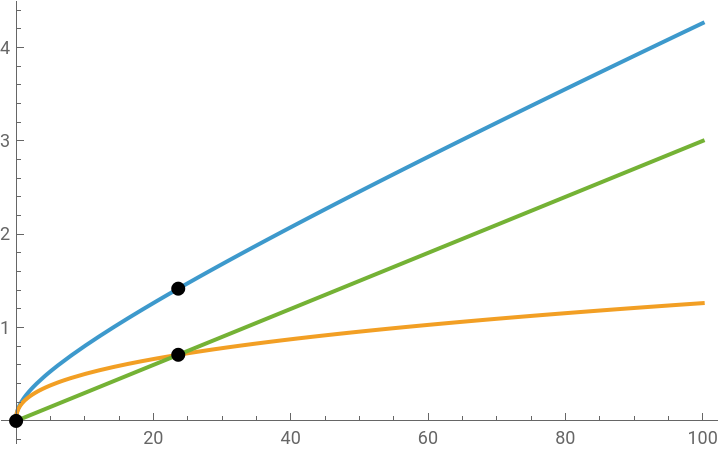
If we further assume that investment per worker is approximated by sk^a where the exponent a is a fixed growth factor (output-capital ratio per worker), we can visualize aggregate output per worker, investment per worker, and the constant depreciation of the productive capital stock per worker by assigning some arbitrary values to the following functions and parameters:
In[]:=
ClearAll[a,s,n,δ,k];s=0.2;a=0.4;n=0.01;δ=0.02;
In[]:=
f[k_]:=sk^a;g[k_]:=(n+δ)k;
The steady state value of the capital stock per worker can be found by setting = 0, which gives sf(k) = (n+δ)k.
k
In[]:=
Solve[f[k]==g[k],k]
Out[]=
{{k0.},{k23.6146}}
From these two values, we can also determine corresponding steady state values of (n+δ)k and of aggregate output per worker by:
In[]:=
g[k]/.k->{0,23.61463487072469`}f[k]+g[k]/.k->{0,23.61463487072469`}
Out[]=
{0.,0.708439}
Out[]=
{0.,1.41688}
In[]:=
Plot[{f[k]+g[k],f[k],g[k]},{k,0,100},PlotLegends->{"Aggregate Output per Worker","Investment per Worker","(n+δ)k"},Epilog->{PointSize[Large],Point[{{0,0},{23.61463487072469`,0.7084390461217407`},{23.61463487072469`,1.4168780922434814`}}]}]
Out[]=


The technology-augmented Solow growth model
The technology-augmented Solow growth model
The specification of aggregate production function and the capital stock growth with A term
The specification of aggregate production function and the capital stock growth with A term
Solow (1957) modified his previous aggregate production function by introducing a new variable A. The aggregate production function with two inputs, the productive capital stock, K, and the effective labor input, AL, is now defined by:
Y=F(K,AL)
(
7
)The growth of the productive capital stock remains the same as before: It is a positive function of aggregate savings and a negative function of a constant depreciation, δ, of the productive capital stock. Therefore, the capital stock changes by:
K
∂K
∂t
(
8
)If we continue to assume that the labor force (i.e., the number of employed workers) grows at the same constant rate, n, as before, and the A term also grows at a constant growth rate of g, then we can specify the growth of labor force by L(t) = , where is the initial value of labor force and the growth of the A term by A(t) = where is the initial value of the A term.
L
0
nt
L
0
A
0
gt
A
0
Replacing and inserting Y and A(t) L(t) into the growth of the capital stock, , we get:
K
K
A
0
gt
L
0
nt
(
9
)The derivation of the intensive form of aggregate production function
The derivation of the intensive form of aggregate production function
Using the same notation for the productive capital stock per effective worker, let us define k ≡ K/AL. Then K = kAL = k. Taking time derivative of the right-hand side of the equation, we get:
A
0
gt
L
0
nt
K
k
A
0
gt
L
0
nt
A
0
gt
L
0
nt
A
0
gt
L
0
nt
k
A
0
gt
L
0
nt
K
The last expression = ( + gk + nk) must equal to sF(K, ) - δK in (9). That is,
K
k
A
0
gt
L
0
nt
A
0
gt
L
0
nt
K
k
A
0
gt
L
0
nt
A
0
gt
L
0
nt
(
10
)Due to constant returns to scale (CRS) assumption, we can safely express the original aggregate production function in terms of the capital stock per effective worker by dividing both sides of the equations by A(t)L(t) = . Then we get:
A
0
gt
L
0
nt
(+gk+nk)=sFK-δK=sf(k)-δk.
k
A
0
gt
L
0
nt
A
0
gt
L
0
nt
(
11
)From the last expression ( + gk + nk) = sf(k) - δk, we can ultimately derive:
k
k
(
12
)The last expression tells us that the growth of the productive capital stock per effective worker is a positive function of investment per effective labor but a negative function of both population growth, the growth of the A term, and the constant depreciation rate of the capital stock per effective labor.
A static visualization of the solution curve with fixed parameters
A static visualization of the solution curve with fixed parameters
As before, let us also visualize the output per effective worker, investment per effective worker, and the constant depreciation of capital stock per effective worker by assigning some arbitrary values to the following functions and parameters. We continue to assume that sf(k) is best approximated by sk^a:
In[]:=
ClearAll[a,s,n,δ,k,h,j];s=0.2;a=0.4;n=0.01;g=0.01;δ=0.02;h[k_]:=sk^a;j[k_]:=(n+g+δ)k;
The steady state value of capital stock per effective worker can be found by setting = 0, which gives sf(k) = (n+g+δ)k.
k
In[]:=
Solve[h[k]==j[k],k]
Out[]=
{{k0.},{k14.6201}}
From these two values, we can also determine corresponding steady state values of (n+g+δ)k and of output per effective worker by:
In[]:=
j[k]/.k->{0,14.62008869106433`}h[k]+j[k]/.k->{0,14.62008869106433`}
Out[]=
{0.,0.584804}
Out[]=
{0.,1.16961}
In[]:=
Plot[{h[k]+j[k],h[k],j[k]},{k,0,100},PlotLegends->{"Output per Effective Worker","Investment per Effective Worker","(n+g+δ)k"},Epilog->{PointSize[Large],Point[{{0,0},{14.62008869106433`,0.5848035476425733`},{14.62008869106433`,1.1696070952851465`}}]}]
Out[]=
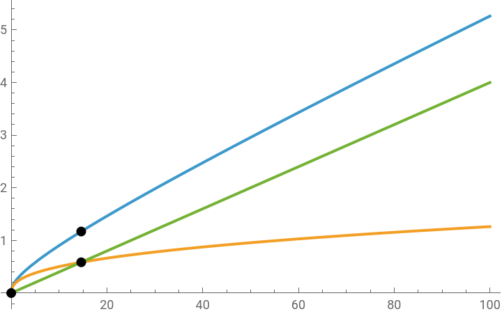
The qualitative behavior of this new model remains the same as before, but the level of each variable is shift upward due to the augmentation by the A-term.
The technology-augmented Solow growth model with a Cobb-Douglas production function
The technology-augmented Solow growth model with a Cobb-Douglas production function
The Cobb-Douglas specification of aggregate production function and the capital stock growth with the A term
The Cobb-Douglas specification of aggregate production function and the capital stock growth with the A term
As a side note, let us introduce a Cobb-Douglas production function. The Cobb-Douglas function used in mathematics has one unique property that satisfies Solow’s fundamental assumption of the constant returns to scale. One example of using this function to represent Solow’s ideas is the following:
Y(t)=F(K,AL)=A(t)KL(whereα+β=1)
α
(t)
β
(t)
(
13
)The growth of the capital stock, the labor force growth, and the growth of the A-term remain the same as before.
The derivation of the intensive form of the Cobb-Douglas aggregate production function
The derivation of the intensive form of the Cobb-Douglas aggregate production function
The last expression in (17) tells us that the growth of the capital stock per effective worker is a positive function of investment per effective labor but a negative function of both population growth, the growth of the A term, and the constant depreciation rate of the capital stock per effective labor, which is exactly the same as we saw in the previous section. The only difference is that this general relationship is now expressed in terms of the Cobb-Douglas function.
Computations with Mathematica
Computations with Mathematica
The above logical inference can be easily verified by the following computations:
Defining functions
Defining functions
The capital stock and its derivative
The capital stock and its derivative
Since k(t) = K(t)/A(t)L(t), K(t) = k(t)A(t)L(t). The function for the capital stock and its time derivative are:
From this, k’(t) is obtained by dividing by A(t)L(t):
Another equation for the derivative of the growth of the capital stock
Another equation for the derivative of the growth of the capital stock
By definition, the growth of the capital stock is given by the equation (14). Dividing this equation by A(t)L(t), we get:
Simplifying the two equations for the capital stock growth
Simplifying the two equations for the capital stock growth
These two equations shows the time derivative of k(t), which must equal to each other. Setting them equal and simplifying further, we get:
The last expression shows how the capital stock per effective worker changes over time. Recall that the constant returns to scale assumption means that α + β = 1. Therefore, β = 1 - α . Replacing β with 1 - α, we get:
The last expression is equal to the equation (17).
An interactive visualization of the technology-augmented Solow growth model
An interactive visualization of the technology-augmented Solow growth model
We can also create a syntax for a dynamic visualization of the Solow growth model. The syntax below generates an interactive chart that allows us to control the parameter for the output per effective worker and investment per effective worker.
For simplicity, we will assume that the population (labor force) does not change. In this case, the average saving rate and the constant depreciation rate are the only crucial parameters that induce the change in the dynamics of both output per effective worker and investment per effective worker.
So-called growth accounting with the Cobb-Douglas function
So-called growth accounting with the Cobb-Douglas function
Total differentials or the chain rule of differentiation
Total differentials or the chain rule of differentiation
Solow’s aggregate production function with the A term can be easily modified into an econometric equation for empirical regression. By taking total differentials of the growth rate of output per effective labor as a function of the growth rate of three inputs (including the growth rate of the A term), we can see that the growth rate of the output per effective worker is decomposed into these three terms. In the literature, this procedure is known as ‘growth accounting’ popularized by Solow himself and later by Mankiw, Romer, and Weil (1992).
The case of the Cobb-Douglas production function
The case of the Cobb-Douglas production function
The rate of change in the aggregate output per effective worker is, therefore, a weighted sum of the relative rates of change in the A term, the capital stock, and the labor input. The weights are, of course, the respective powers, 1, a, and b.
We can confirm this result by using a function Dt in Mathematica:
Conclusion
Conclusion
This notebook has sought to demonstrate how we can replicate the two Solow growth models by setting up the aggregate production function with/without a specification of the A term. The intensive form of this production function is readily attainable once we impose the constant returns to scale assumption to the aggregate production function.
Using the Cobb-Douglas function as an example, we also attempts to visualize the behavior of the steady state value and the relationship among the output per effective labor, investment per effective labor, and the constant diminution of the capital stock per effective labor associated with the growth rate of population, the A term, and depreciation.
Finally, we have also examined how we can easily modify the technology-augmented Solow growth model into an econometric model to be used to estimate relative growth rate components in and across the country. This modification is a mere application of the chain rule of differentiation to the initial aggregate production function.
One important source of controversy lies in the meaning of the A term. Solow and his followers have interpreted the A term as something to do with the production technology that directly affects the shift of aggregate output per effective labor. Later economists have attempted to (1) introduce a stochastic term inside the A-term (a la the RBC model) and (2) explain the growth of the A-term as a result of the representative firm’s intentional efforts to invent and apply this innovative production technology to the production of final consumption goods (a la Paul Romer’s endogenous growth model). Other groups of economists have rejected this conventional interpretation of the A-term and attempted to explain that it is a merely a result of algebraic derivation based upon a certain unjustifiable assumption. We will examine these divergent interpretations of the A-term and different growth model strategies in upcoming sessions.
Reference
Reference
◼
David Romer, Advanced Macroeconomics, New Jersey: McGraw-Hill (4th edition), 2011.
◼
Nicholas G. Mankiw, David Romer, and David N. Weil, “A Contribution to the Empirics of Economic Growth,” Quarterly Journal of Economics, Vol. 107, No. 2 (1992), pp.407-437.
◼
Robert M. Solow, “A Contribution to the Theory of Economic Growth,” The Quarterly Journal of Economics, Vol. 70, No. 1 (Feb., 1956), pp.65-94.
◼
----------------------, “Technical Change and the Aggregate Production Function," The Review of Economics and Statistics, Vol. 39, No. 3 (Aug., 1957), pp.312-320.
CITE THIS NOTEBOOK
CITE THIS NOTEBOOK
Introduction to dynamic economic models: the Solow growth models
by Hee-Young Shin
Wolfram Community, STAFF PICKS, January 8, 2026
https://community.wolfram.com/groups/-/m/t/3602661
by Hee-Young Shin
Wolfram Community, STAFF PICKS, January 8, 2026
https://community.wolfram.com/groups/-/m/t/3602661