ABSTRACT (original report): This project explores the theta invariant, a powerful, genuinely computable invariant for knots developed by Dror Bar-Natan and Roland van der Veen. We calculate this invariant for several families of knots, including torus, pretzel, and twisted torus knots, to search for the information it holds.
Original report: https://wolfr.am/Theta_Report
Theta Invariant paper: https://doi.org/10.48550/arXiv.2509.18456
Original report code: https://github.com/AliKarimLalani/theta_invariant
Theta Invariant paper code: https://drorbn.net/AcademicPensieve/Projects/Theta/
Quanta Magazine: https://wolfr.am/Quanta_Theta_Invariant
A knot, in the mathematical sense, is a closed loop embedded in three-dimensional space — a circle tangled up in , with its ends joined so no motion can untie it. To study knots concretely, one projects them onto a plane to obtain a knot diagram, a planar picture recording where strands cross over and under one another. The number and arrangement of these crossings encode the topology, but the same knot admits infinitely many diagrams, so comparing diagrams by inspection is unreliable. A knot invariant resolves this: it is a quantity assigned to a knot, not just a diagram, that remains unchanged under any continuous deformation. If two knots yield different invariant values, they are provably distinct. The central challenge in knot theory is to find invariants that are both discriminating and computationally tractable.
3
R
That challenge has defined the field's history. The strongest invariants — Khovanov homology, the HOMFLY-PT polynomial, hyperbolic volume — have high separation power: on knots with up to 15 crossings, Khovanov homology and hyperbolic volume together leave a deficit of roughly 41,000 undistinguished pairs. Yet for most of them, computing the invariant on a knot with 300 crossings is, as Bar-Natan put it, "science fiction." At the other end of the spectrum sits the Alexander polynomial , discovered in 1923: fast to compute, topologically meaningful (it bounds the knot genus and detects fiberedness), yet weak as a separator, its deficit on knots with up to 15 crossings exceeds 236,000. In 2025, Dror Bar-Natan and Roland van der Veen resolved this trade-off with the Theta invariant Θ, introduced in their paper: Dror Bar-Natan, Roland van der Veen, A Fast, Strong, Topologically Meaningful and Fun Knot Invariant, arXiv:2509.18456 (2025).
Δ(T)
Θ achieves a separation deficit below 7,000 on knots with up to 15 crossings — roughly a sixth of everything else combined — while remaining computable in polynomial time, including on knots exceeding 300 crossings. The result was covered in a dedicated article in Quanta Magazine: Erica Klarreich, "A Powerful New QR Code Untangles Math's Knottiest Knots", April 22, 2026.
Θ is a pair . The first component is precisely the classical Alexander polynomial, a one-variable Laurent polynomial in . The second component (,) is a two-variable Laurent polynomial that extends and refines it; Θ is computed by a formula involving the inverse of a matrix built from the crossing data of an -crossing diagram. The bottleneck is inverting , which requires operations in — polynomial time, feasible even when is in the hundreds. To feed a knot to this algorithm, one needs a machine-readable description of its diagram. Planar diagram (PD) notation records each crossing as a tuple , where the four integers label the edge segments at that crossing in cyclic order: incoming under-strand, outgoing over-strand, outgoing under-strand, incoming over-strand. Every edge label appears exactly twice across the full list, encoding the diagram's connectivity. An alternative is braid representation , which describes the knot as the closure of a braid on strands; by Alexander's theorem every knot admits such a representation, and it is often more natural for families defined by repeated twisting.
(Δ,)
Θ
2
Δ(T)
T
Θ
2
T
1
T
2
(2n+1)(2n+1)
A
n
A
O()
3
n
Q(T)
n
X[a,b,c,d]
BR(k,{})
σ
i
k
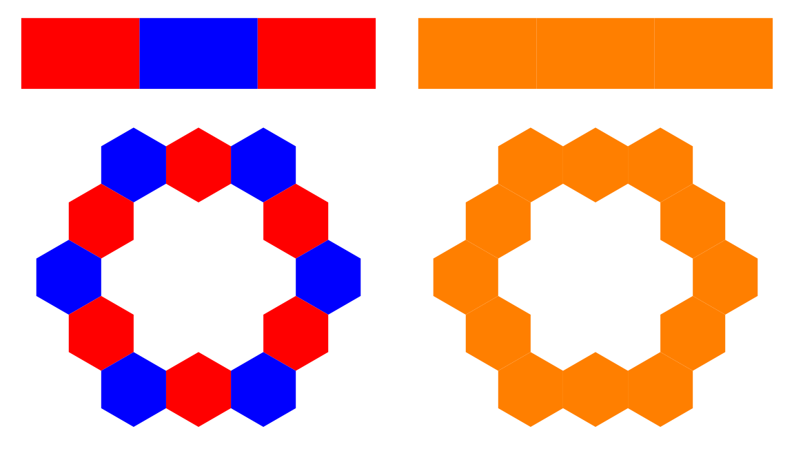
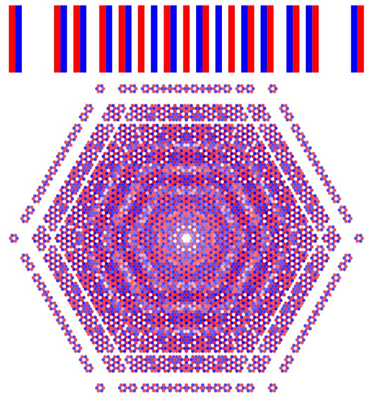
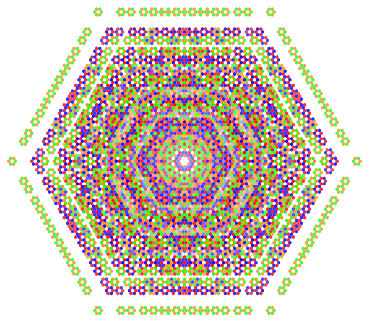
Each pair is visualised as a pair of coefficient diagrams. For , the coefficients indexed by the exponent of form a horizontal bar code, with red cells for positive and blue for negative coefficients. For , the monomial is placed at the sheared grid position -,, turning the support of the polynomial into a hexagonal array of coloured cells. The shear is chosen to make a conjectured hexagonal symmetry of visually apparent. These pictures are called hexagonal QR codes: not literal QR codes in any encoding sense, but geometric visualisations of polynomial coefficients in which algebraic structure — sign, parity, support shape, and symmetry — is directly readable as colour, pattern, and geometry. A ParityPlot variant encodes the parity (odd or even) of each coefficient rather than its sign, and a RainbowPlot encodes all four sign-parity classes simultaneously with logarithmic intensity scaling.
(Δ,)
Θ
2
Δ
T
Θ
2
c·
n
1
T
1
n
2
T
2
n
1
n
2
2
3
2
n
2
Θ
2
This notebook is computational and exploratory. It applies Θ to specific families of knots — torus knots, twist knots, twisted torus knots, and pretzel knots — to observe the visual and algebraic patterns in their hexagonal QR codes and to record conjectural behaviour as explicit formulas or geometric observations. The goal is to document what Θ actually does on structured families at scale, producing conjectures about degree, coefficient polynomials, symmetry violations, and the presence or absence of features such as vanishing constant terms or checkerboard regions.
Backend Code and Helpers for the Invariant
Backend Code and Helpers for the Invariant
All computation uses the KnotTheory package for Mathematica, which provides pre-defined knots, braid and PD conversion, and basic knot operations. The package must reside in the same directory as the notebook before loading.
(* Importing Dror's Package*)SetDirectory[NotebookDirectory[]];<<KnotTheory`
Loading KnotTheory` version of October 29, 2024, 10:29:52.1301.Read more at http://katlas.org/wiki/KnotTheory.
Technical Helper
Technical Helper
Main Program
Main Program
Θ[K_]
K
Rot
A
det(A)
A
G
ev
(Δ,θ)
θ·
Δ
1
Δ
2
Δ
3
θ
0
A
(2n+1)(2n+1)
T
O()
3
n
In[]:=
Θ[K_] := Module[{Cs, φ, n, A, Δ, G, ev, θ}, {Cs, φ} = Rot[K]; n = Length[Cs]; A = IdentityMatrix[2*n + 1]; Cases[Cs, {s_, i_, j_} :> (A[[{i, j}, {i + 1, j + 1}]] += {{-T^s, T^s - 1}, {0, -1}})]; Δ = T^((-Total[φ] - Total[Cs[[All, 1]]])/2)*Det[A]; G = Inverse[A]; ev[ℰ_] := Factor[ℰ /. Subscript[g, ν_, α_, β_] :> (G[[α, β]] /. T -> Subscript[T, ν])]; θ = ev[Sum[Subscript[R, 12][Cs[[k1]], Cs[[k2]]], {k1, 1, n}, {k2, 1, n}]]; θ += ev[Sum[Subscript[R, 11][Cs[[k]]], {k, 1, n}]]; θ += ev[Sum[Subscript[Γ, 1][φ[[k]], k], {k, 1, 2*n}]]; Factor[{Δ, (Δ /. T -> Subscript[T, 1])*(Δ /. T -> Subscript[T, 2])*(Δ /. T -> Subscript[T, 3])*θ}]];
The output is the pair as Mathematica expressions in and respectively, ready to be passed directly to the plotting routines or expanded for coefficient extraction.
(Δ,θ)
T
(,)
T
1
T
2
We compute Θ on the trefoil knot as a first check:
In[]:=
trefoil=Knot[3,1];trefoilΘ=Θ[trefoil]
Out[]=
,-
1-T+
2
T
T
1-+--++--+-+
T
1
2
T
1
T
2
3
T
1
T
2
2
T
2
4
T
1
2
T
2
T
1
3
T
2
4
T
1
3
T
2
2
T
1
4
T
2
3
T
1
4
T
2
4
T
1
4
T
2
2
T
1
2
T
2
Plotting Tools
Plotting Tools
Some Computations
Some Computations
We compute Θ on the trefoil and display its PolyPlot and ParityPlot side by side. The hexagonal support and the all-orange ParityPlot (all coefficients of θ are odd and equal to ±1 for the trefoil) are consistent with the conjectured symmetry structure.
In[]:=
GraphicsRow[{PolyPlot[trefoilΘ], ParityPlot[trefoilΘ]}, ImageSize -> Large]
Out[]=
(10,7) Torus Knot
(10,7) Torus Knot
In[]:=
AbsoluteTiming[T107=Θ[TorusKnot[10,7]];]PolyPlot[T107]
Out[]=
{30.7264,Null}
Out[]=
In[]:=
RainbowPlot[T107]
Out[]=
The Rolfsen Table
The Rolfsen Table
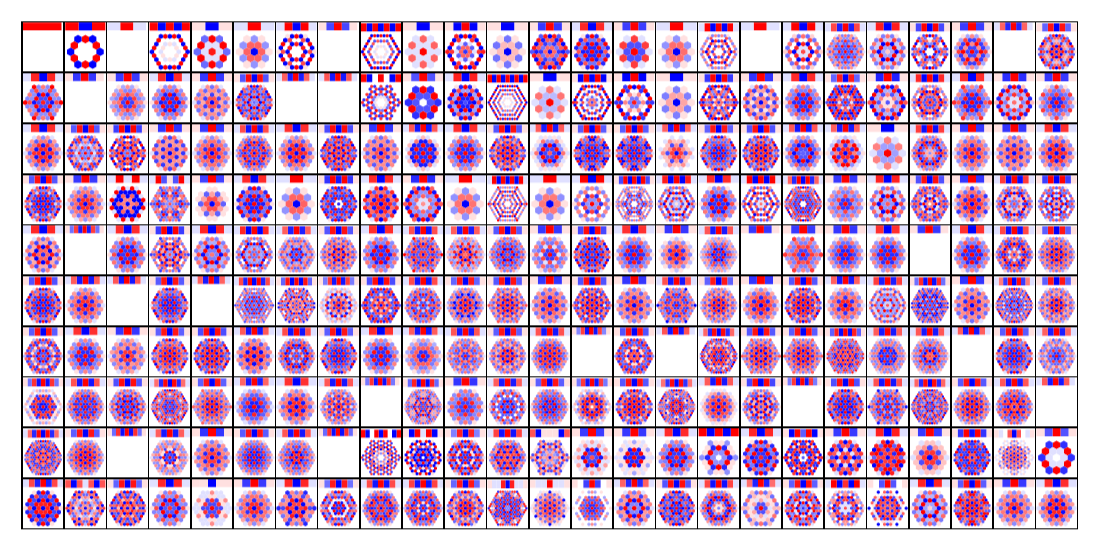
We run Θ on every prime knot with at most 10 crossings (the Rolfsen table) and display the PolyPlot and ParityPlot grids. The grid provides a visual census: each cell is the coefficient picture of one knot. Comparing cells across the grid reveals which knots share structural features of their theta polynomials and which are visually and algebraically isolated.
In[]:=
(* Data for ther first 250 Prime Knots *)tab250 = {{1, 0}} ~Join~ Table[Θ[K], {K, AllKnots[{3, 10}]}];GraphicsGrid[Partition[PolyPlot /@ tab250, 25], Spacings -> 0, Dividers -> All]GraphicsGrid[Partition[ParityPlot /@ tab250, 25], Spacings -> 0, Dividers -> All]
Out[]=
Representing Families of Knots
Representing Families of Knots
In this section, we formally define the families of knots investigated in this project. For each family, we provide a brief description and the corresponding implementation code.
Torus Knots
Torus Knots
Twist Knots
Twist Knots
1
.Two clasp crossings that form the upper loop of the knot.
2
.A series of n twist crossings that form the right-handed ”rungs” of the lower twisted section.
3
.A series of connecting crossings that form the ”rails” linking the twists together.
Pretzel Knots
Pretzel Knots
We generate the planar diagram by defining each crossing according to a geometric labeling. The code first defines a set of helper functions that permute the arguments of a crossing X[a,b,c,d] to handle the four possible crossing orientations. The choice of orientation for each crossing in a tangle depends on two factors: the sign of its parameter pi (determining right- or left-handed twists) and the parity of the tangle’s index i (determining how it weaves into the main loops).
The main function then assembles the knot by building three distinct lists of crossings:
(1) Interior Crossings: A list of crossings forming the internal ”rungs” of each tangle. These are represented via lc (left columns) and rc (right columns) respectively.
Finally, these lists are combined and processed by CanonicalPD function to produce a unique representation of the knot. We include the code in the case where n is even below, and WLOG the even parameter is the first one.
CITE THIS NOTEBOOK
CITE THIS NOTEBOOK
A computational survey of the Theta invariant
by Ali Karim Lalani
Wolfram Community, STAFF PICKS, May 11, 2026
https://community.wolfram.com/groups/-/m/t/3714716
by Ali Karim Lalani
Wolfram Community, STAFF PICKS, May 11, 2026
https://community.wolfram.com/groups/-/m/t/3714716