The whole idea in one image. Each sextant sight places you on a circle of equal altitude drawn on the Earth; three such circles sweep across the globe and converge on your position — the glowing fix. This post derives that geometry from first principles and measures exactly how well it works. Built entirely offline; the star field and Milky Way are for atmosphere.
A complete Wolfram Language implementation of celestial navigation: sextant corrections, sight reduction, running fixes, star selection, Cramér–Rao bounds, lunar-distance longitude, a recursive Kalman fix, and a simulated Atlantic passage — all code loaded from two .wl packages and shown above every result.
Abstract
Abstract
On a clear night at sea, three star observations with a sextant and a reliable clock fix your position to about 1 nautical mile (nm) — but only the random part of the error averages down to 1 nm; the systematic part (index error, refraction model, almanac) does not, so real fixes are usually 1–3 nm and sometimes worse. GPS does the same job to 5 m. Both are elegant: GPS triangulates from radio signals from 24 satellites; the sextant triangulates from ancient starlight and spherical geometry. This post builds the entire method from first principles in Wolfram Language.
All code lives in two package files — CelestialNavigation.wl (the engine) and SextantFigures.wl (the figures) — which the notebook loads with Get. Above every figure and every computed number you will see the exact function call that produced it, so the whole post is re-runnable.
Topics: sextant altitude corrections; the Marcq St–Hilaire intercept method; running fixes and the cocked hat; the 57-star navigational catalogue with IAU-1976 precession; optimal star selection by GDOP; the Cramér–Rao lower bound; the Daniels 1951 cocked-hat 25 % theorem; the lunar-distance method for finding GMT without a chronometer; a recursive (Kalman) running fix; offline ephemeris validation; and a reconstruction of Shackleton's 1916 James Caird voyage. Everything runs offline.
Audience: the narrative assumes high-school trigonometry and a passing curiosity about ships. Each section opens with an intuitive explanation, then deepens into the exact formulae in the package.
Setup (optional — only needed to re-evaluate code cells)
Setup (optional — only needed to re-evaluate code cells)
You can skip this section entirely if you only want to read. Every figure and every code output is pre-computed, so the prose, equations, figures, and numbers all work without evaluating anything.
To run the code cells yourself, place CelestialNavigation.wl, SextantFigures.wl, and SextantInteractive.wl (all three uploaded alongside the notebook) in the same folder as the .nb file, then evaluate:
SetDirectory[NotebookDirectory[]];Get["CelestialNavigation.wl"];Get["SextantFigures.wl"];Get["SextantInteractive.wl"];Print["engine v",cnVersion[]," / ",sxFigVersion[]," / ",sxManipVersion[]]
The engine defines the cn... functions (the mathematics); the figures package defines 27 sxFig...[] functions, each returning a finished graphic; and SextantInteractive.wl defines the three live sxManip...[] demonstrations of §14. Re-evaluating any sxFig...[] cell regenerates that figure from scratch.
1. The Problem of Position
1. The Problem of Position
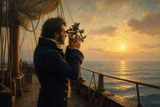
AI-generated illustration (OpenAI gpt-image-2) — for atmosphere, not a data figure. The human act at the heart of the method: a navigator brings a star down to the horizon with a sextant. Everything that follows turns that single measured angle into a position.
Latitude was easy. The elevation of Polaris above the northern horizon equals your latitude to within a degree. A noon Sun observation gives it more precisely: latitude = declination + zenith distance of the Sun at its highest point. These methods need no clock at all, just a sextant and an almanac.
Longitude was hard. Earth rotates once every 24 hours, so every 4 seconds of time corresponds to 1 nautical mile of longitude error at the equator. Before the Harrison chronometer (H4, 1759), no clock at sea was accurate enough for longitude. The 1714 Longitude Act offered £20,000 (about £3 M today) to anyone who solved the problem.
Two key methods emerged. Thomas Sumner (1837) accidentally discovered the circle of equal altitude: every observer on the same circle around the sub-stellar point sees the same star altitude. Marcq St–Hilaire (1875) turned two or more such circles into an operational fix by the intercept method, still taught to every maritime candidate today.
The cover animation above is the thesis of this whole post: a celestial navigator, armed only with a sextant, a watch, and spherical trigonometry, holds position to within a couple of nautical miles across an ocean crossing. The rest of the post derives exactly how, and exactly how well.
2. The Celestial Sphere & Coordinates
2. The Celestial Sphere & Coordinates

AI-generated illustration (OpenAI gpt-image-2) — for atmosphere, not a data figure. The celestial dome over the observer: stars fixed on an imaginary sphere of infinite radius, each reduced to two angles — altitude above the horizon and azimuth around it.
The celestial sphere is an imaginary sphere of infinite radius centred on Earth. Every celestial body is projected onto it. An observer's view reduces to two angles: altitude H (degrees above the horizon, 0°–90°) and azimuth Zn (bearing clockwise from North, 0°–360°).
A body's position on the sphere is fixed by its declination δ (celestial latitude) and its Greenwich Hour Angle (GHA): the angle westward from the Greenwich meridian to the body's meridian. For stars the catalogue gives Sidereal Hour Angle (SHA) measured from the First Point of Aries (♈), and GHA = GAST − SHA (mod 360°).
GHA=GAST-SHA(mod360°)
The Sun's sub-solar point (geographic position, GP) is the point on Earth's surface where the Sun is directly overhead. Its latitude equals the solar declination and its longitude is −GHA. For 22 Nov 2024 at 12:00 UTC:
cnSunGP[DateObject[{2024,11,22,12,0,0},TimeZone->0]]
{-20.2897,-3.43836}
Result: {declination °, GP longitude °}. The Sun's declination on 22 Nov 2024 is near −20° (the northern winter approach).
sxFigCelestialSphere[]
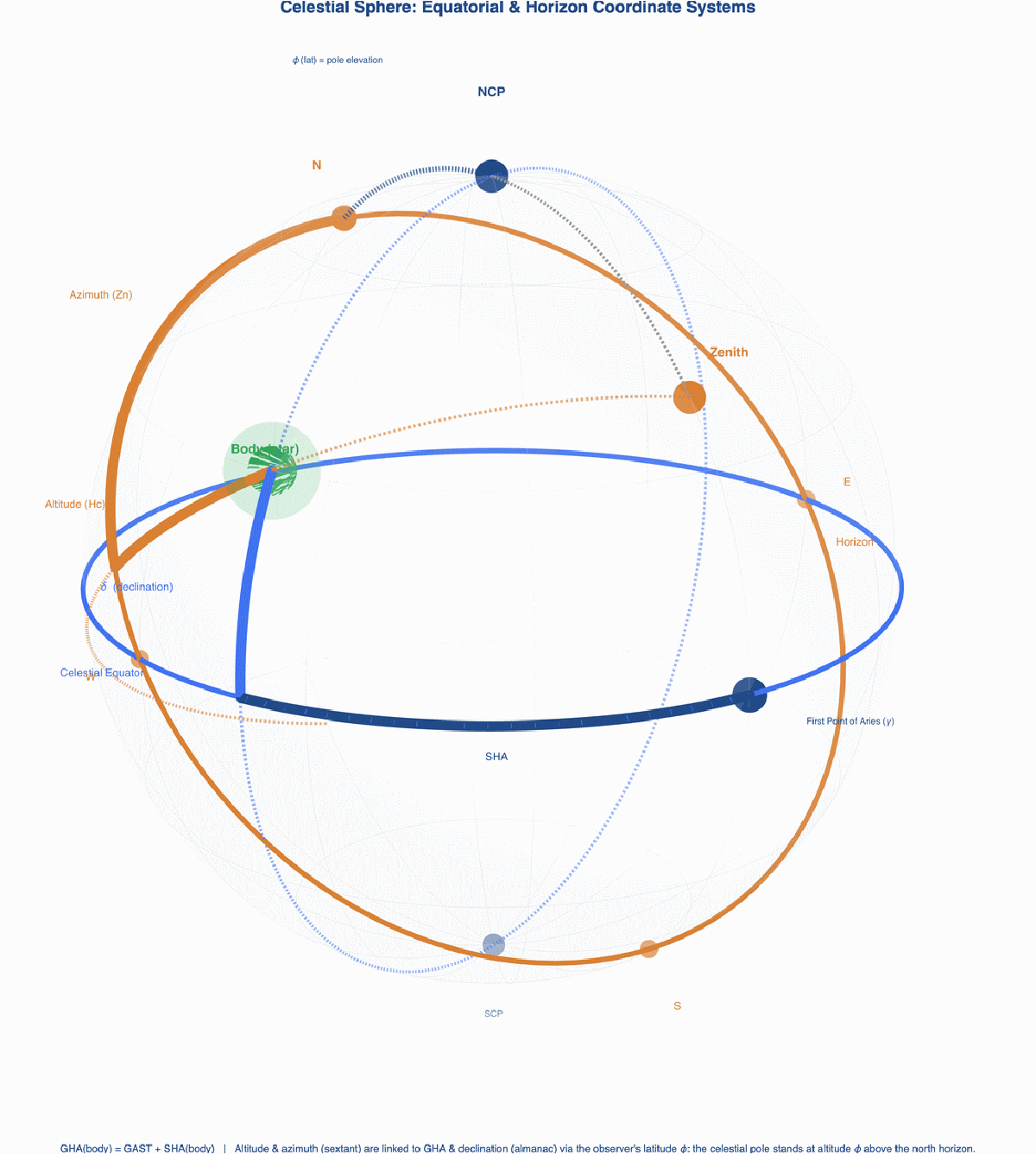
Figure 2.1 The celestial sphere, showing the observer's zenith Z, the body X, the celestial pole P, and the navigational triangle PZX. The altitude H is the complement of the zenith distance z = 90° − H.
sxFigEquationOfTime[]
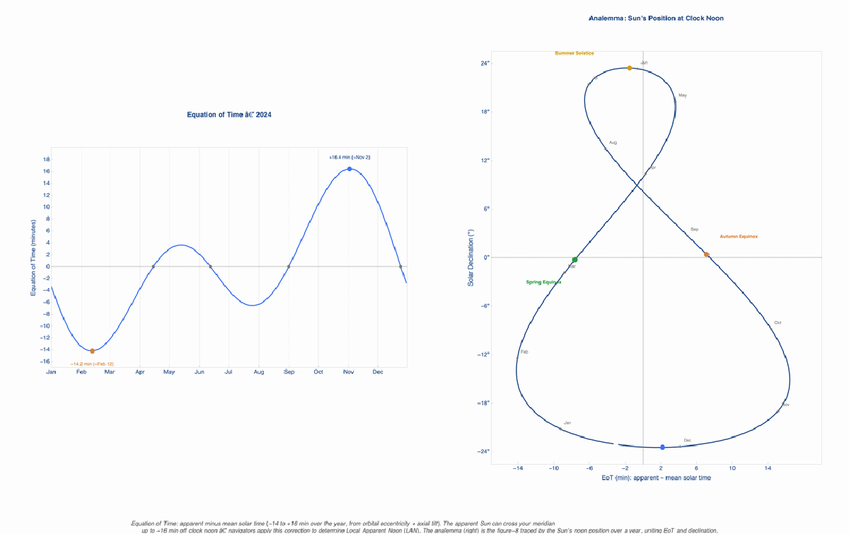
Figure 2.2 The equation of time (EoT) and the analemma. EoT = apparent solar time − mean solar time, ranging ± 16 minutes. The analemma is the figure-eight traced by the Sun at a fixed clock time through the year.
sxFigSubsolarTrack[]
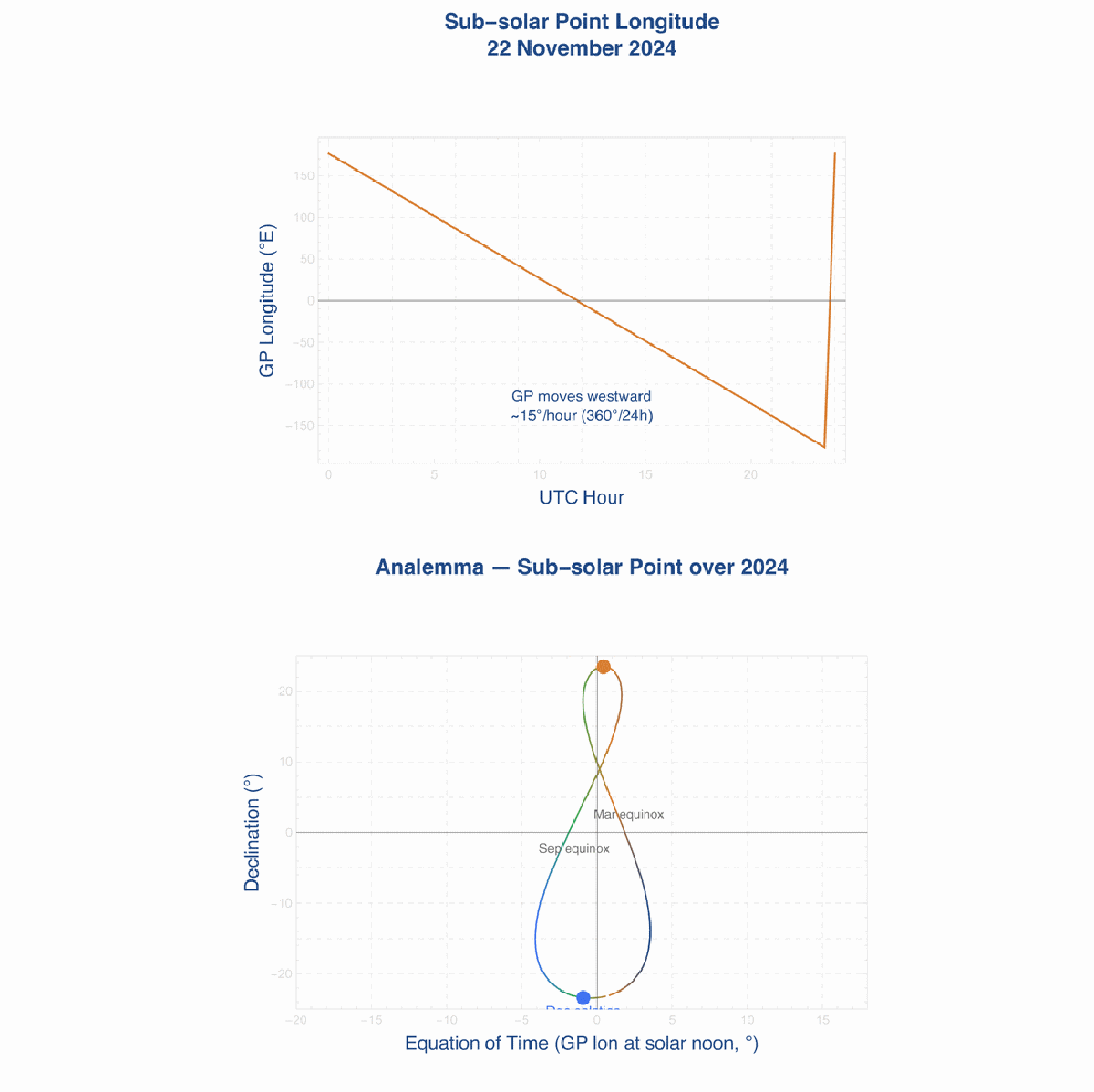
Figure 2.3 Sub-solar point track over 24 hours (22 Nov 2024). The latitude band is set by solar declination; the longitude sweeps 360° in 24 hours as Earth rotates.
3. A Sight Is a Circle
3. A Sight Is a Circle
When you measure the Sun's altitude H = 45° with a sextant, you know only that you lie somewhere on a circle of equal altitude: a circle on Earth's surface centred on the GP of the Sun, with angular radius 90° − H = 45°. That circle has radius 45° × 60 = 2700 nm — you are a long way from being exactly located.
The altitude at any observer position {lat, lon} from a body at GP {dec, lon⎵GP} follows directly from the spherical law of cosines:
where ϕ is observer latitude, δ is declination, and LHA = lon⎵observer − lon⎵GP. At {35°N, 15°W} and the sub-solar GP computed above:
Result: the geometric altitude of the Sun in degrees — the ideal sextant reading before any instrument corrections.
Figure 3.1 The circle of equal altitude centred on the GP. Two circles narrow the fix to two points; a third disambiguates. This is the conceptual foundation of celestial navigation.
4. The Sextant and Its Corrections
4. The Sextant and Its Corrections
A sextant measures the angle between a celestial body and the visible horizon. The reading H⎵s (sextant altitude) differs from the true observed altitude H⎵o by five systematic corrections:
• Index error (IE): instrument calibration offset, measured by the navigator.
• Refraction: the atmosphere bends light downward. Bennett (1982): R = cot(H + 7.31/(H+4.4)) arcmin. Subtract. At 45°, R ≈ 1'.
• Semi-diameter (SD): the Sun and Moon are discs; navigators sight a limb. Add/subtract ≈16' for lower/upper limb.
• Parallax (HP): the Sun is not infinitely far; HP ≈ 0.15·cos(H) arcmin. Add.
For a sextant reading of 45°, eye height 2 m, no index error, lower limb:
Result: observed altitude H⎵o in degrees. The net correction is about −0.03° (−2') — dip and refraction dominate here.
Figure 4.1 Waterfall chart of sextant corrections for a Sun lower-limb sight at 45°, 2 m eye height. Each bar is one correction; the net gives H⎵o.
Figure 4.2 Atmospheric refraction vs altitude (Bennett 1982, Saemundsson 1986, and the simple cot model). Refraction diverges near the horizon and is below 1' above 45°.
Figure 4.3 Horizon dip vs eye height. At 2 m (small-boat deck) dip ≈ 2.5'; at 15 m (ship's bridge) dip ≈ 6.8'.
5. The Navigational Triangle
5. The Navigational Triangle
Three special points define a spherical triangle for each observation: the elevated Pole P, the observer's Zenith Z, and the body X. This is the navigational triangle PZX.
Its three sides carry the key angles: PZ = co-latitude (90°−ϕ), ZX = zenith distance (90°−H), and PX = polar distance (90°−δ). The angle at P equals the Local Hour Angle (LHA). The spherical law of cosines on side ZX gives the fundamental equation of sight reduction:
Given an assumed position {lat, lon} and the body's GP, it gives the computed altitude H⎵c and azimuth Zn. At the demo position:
Result: {H⎵c °, Zn °}. The Sun bears roughly south (Zn near 180°) in the northern hemisphere near noon.
Figure 5.1 The PZX navigational triangle on the celestial sphere. The law of cosines on side ZX yields sin H = sin ϕ sin δ + cos ϕ cos δ cos LHA.
6. Sight Reduction — The Intercept Method
6. Sight Reduction — The Intercept Method
The Marcq St–Hilaire (1875) intercept method turns a single sextant observation into a line of position (LOP):
(1) Choose an assumed position (AP) near your DR position. (2) Compute H⎵c and Zn from the AP. (3) The intercept is a = (H⎵o − H⎵c)×60 nm (positive = toward the body). (4) Plot a line perpendicular to Zn at distance a from the AP.
One observation with a deliberate 0.05° (3 nm) positive intercept:
Result: an Association with keys AP, Hc, Zn, Ho, interceptNm (positive = Toward), point (closest point on the LOP to the GP), and bearingDeg. With Ho > Hc by 0.05°, the LOP sits 3 nm toward the Sun from the AP.
Figure 6.1 The intercept method. AP is the assumed position; a is the intercept (positive = toward the body). The LOP is drawn perpendicular to the azimuth Zn at distance a from AP.
7. One Line Is Not a Fix — Running Fix & Cocked Hat
7. One Line Is Not a Fix — Running Fix & Cocked Hat
A single LOP tells you which line you are on, not where on it. Two simultaneous LOPs from well-separated bodies fix the position at their intersection. With only the Sun by day, you must use a running fix: advance the morning LOP along your course and speed to the time of the afternoon sight, then intersect.
Three LOPs rarely meet at one point — errors produce a cocked hat (triangle). Daniels (1951) proved that, for any symmetric error distribution, the true position lies inside the cocked hat with probability exactly 25 % (revisited in §9).
Running fix from two Sun sights (08:00 and 12:00 UTC, advancing the morning LOP 20 nm on course 270°):
Result: {latitude, longitude} of the running fix in degrees. With near-zero sextant noise the fix recovers the true position to within a few tenths of a nm; realistic 1' sextant noise translates to ~1 nm.
Figure 7.1 Running-fix geometry. The morning LOP is advanced along the course track to the time of the noon sight (the transferred position line); its intersection with the noon LOP is the running fix.
Figure 7.2 A cocked-hat triangle from three Sun LOPs with realistic 1'-noise sextant errors. The three pairwise intersections form the triangle; the true position lies inside with probability 25 % (Daniels 1951).
8. Real Stars at Twilight
8. Real Stars at Twilight
Astronomical twilight (Sun 12°–18° below the horizon) is the navigator's golden window: the horizon is still sharp, yet bright stars are visible. In this ~20-minute window, three to five star LOPs can be reduced to a simultaneous fix.
The package carries all 57 navigational stars (J2000.0 right ascension, declination, magnitude) with full IAU-1976 precession to the date of observation. A good triplet needs three stars well above the horizon, evenly spaced in azimuth (ideally 120° apart), and bright enough to measure.
Result: <|"stars" -> {n1, n2, n3}, "gdop" -> _, "azimuths" -> {Az1, Az2, Az3}|>. A GDOP near 1.15 means near-optimal spacing.
The GDOP of that chosen triplet, evaluated directly:
Result: the scalar GDOP for that star set — it matches the "gdop" key above.
With zero-noise LOPs from those three stars, the least-squares intersection cnFix recovers the true position exactly:
Result: {latitude, longitude}. The three exact LOPs intersect at {15°N, 40°W}, confirming the reduction is self-consistent.
Figure 8.1 Twilight sky at the demo position (15°N, 40°W, 21 Jun 2025 22:00 UTC). Navigational stars above 15° are plotted on an altitude-azimuth grid; the optimal (best-GDOP) triplet is highlighted.
Figure 8.2 GDOP as the third star is varied (best two fixed). Lower GDOP = better geometry; the optimal choice fills the azimuth gap.
Figure 8.3 Replay of one evening twilight star fix. Three star LOPs form a small cocked hat; the fix lands within ~1 nm of GPS truth, consistent with 1' sextant noise and a low GDOP.
9. How Good Is It? The Statistics
9. How Good Is It? The Statistics
Three non-obvious statistical results about celestial navigation — and one honest caveat that frames the rest of the post.
9.1 The Cocked-Hat 25 % Theorem
9.1 The Cocked-Hat 25 % Theorem
Daniels (1951) proved that for any three LOPs with any symmetric error distribution (not just Gaussian), the probability that the true position lies inside the cocked-hat triangle is exactly 25 %. Monte-Carlo over noisy three-star fixes confirms it:
Result: the empirical fraction of trials with the true position inside the cocked hat — close to 0.25, independent of the noise amplitude. A small cocked hat is therefore reassuring but NOT proof you are inside it.
Figure 9.1 Monte-Carlo verification of the 25 % theorem (10 000 trials). The inside-fraction converges to 0.25 (dashed line) regardless of noise amplitude.
9.2 Cramér–Rao Lower Bound
9.2 Cramér–Rao Lower Bound
The Fisher information matrix from LOPs with azimuths {Zn⎵i} and sight noise σ (arcmin = nm) is:
The Cramér–Rao bound says no unbiased estimator beats F^{-1} in position variance. For three stars at 45°, 165°, 285° (near-optimal 120° spacing) with 1' sigma:
Result: <|semiMajorNm, semiMinorNm, orientDeg, cep|>. With near-optimal geometry and 1' noise the CRLB predicts CEP ≈ 0.8–1.0 nm — this is the RANDOM-NOISE FLOOR under a perfect ephemeris, not the real-world error.
Figure 9.2 CRLB covariance ellipse vs Monte-Carlo fix scatter (1' noise). The Monte-Carlo ellipse matches the CRLB, confirming the sight-reduction algorithm is near-optimal for random noise.
Figure 9.3 Error ellipses for different star-triplet geometries. Near-optimal 120° spacing gives a round ellipse (CEP ≈ 0.9 nm); clustered geometry gives an elongated ellipse whose worst axis exceeds 5 nm.
9.3 Dilution of Precision
9.3 Dilution of Precision
The honest floor. The ~1 nm CRLB/Monte-Carlo number is the random-noise floor assuming a perfect ephemeris. Real fixes are dominated by systematic error — index error, the refraction model, almanac residuals — which does not average out over several sights. Real-world celestial fixes are typically 1–3 nm, and worse in poor conditions. §12 makes this explicit.
9.4 The Full Picture: the Bayesian Position Posterior
9.4 The Full Picture: the Bayesian Position Posterior
The MAP (maximum-a-posteriori) estimate for three clean Sun sights at the demo truth {20°N, 40°W}:
Result: {lat, lon} of the posterior peak — it lands on the true position {20°N, 40°W} to within the grid resolution, confirming three clean sights concentrate the posterior on the truth.
Figure 9.5 The Bayesian position posterior. One sight is a fuzzy BAND (the line of position as a likelihood ridge); two sights a BLOB; three a tight PEAK on the true position. The fourth panel bakes in a constant uncorrected index error: the peak stays tight but shifts OFF the truth — the honest, complete picture of why scatter is not accuracy.
10. The Longitude Problem & Lunar Distance
10. The Longitude Problem & Lunar Distance
AI-generated illustration (OpenAI gpt-image-2) — for atmosphere, not a data figure. The clock solution: a Harrison-style marine chronometer. Keeping exact Greenwich time at sea turned longitude from an unsolved problem into a single subtraction.
The 4-second rule. Earth rotates 360° in 24 hours = 15 arcmin per second. Since 1 arcmin of longitude at the equator = 1 nm, every second of chronometer error is 0.25 nm of longitude error at the equator (scaled by cos(lat)). This is exactly why Harrison's H4 mattered:
Result: 0.25 nm per second at the equator — 4 seconds = 1 nm. At latitude 45° it is 0.25 cos(45°) ≈ 0.177 nm/s.
Figure 10.1 Longitude error vs chronometer error at three latitudes. The equatorial slope is exactly 0.25 nm/s. H4 was good to ~0.2 s/day — comfortably inside the Longitude Board's 1-nm-per-day standard.
Latitude is immune to clock error. At Local Apparent Noon the Sun transits the meridian at maximum altitude; only that maximum value is needed, not absolute time:
Result: observer latitude. With Ho = 50° and δ = −20°, z = 40° and lat = δ + z = 20°N.
Figure 10.2 Sun altitude vs UTC near Local Apparent Noon. The flat ~2-minute-wide peak limits noon-latitude precision to about ±0.02° (±1.2').
10.1 Longitude Without a Chronometer: Lunar Distance
10.1 Longitude Without a Chronometer: Lunar Distance
AI-generated illustration (OpenAI gpt-image-2) — for atmosphere, not a data figure. The no-clock method: measuring the angular distance between the Moon and the Sun. The Moon drifts ~0.5° per hour against the stars, so that angle is itself a slow clock in the sky.
Before reliable chronometers, navigators found GMT from the lunar distance — the angle between the Moon and the Sun (or a star). The Moon moves ~0.5°/hour against the background, so the Moon-Sun distance is a slow clock in the sky. The geocentric distance at a given instant:
Result: the center-of-Earth Moon-Sun angular distance in degrees.
A real observation is topocentric and refracted; it must be cleared to the geocentric value before it can be used. Given the observed distance and the apparent Moon/Sun altitudes:
Result: the cleared (geocentric) distance — it should match cnLunarDistanceGeocentric above to within the sextant noise.
Inverting the monotonic distance-vs-time relation recovers GMT:
Result: the recovered UTC, near the true 18:00. In practice a 1' error in the cleared distance maps to ~2 minutes of time — about 0.5° (~30 nm) of longitude. Lunars are far coarser than a chronometer (4 s = 1 nm) — which is precisely why Harrison's clock won.
Figure 10.3 Left: the Moon-Sun distance as a clock (~0.5°/hr), inverted to recover GMT. Right: the resulting longitude error vs lunar-distance measurement error — tens of nautical miles, the historical reality.
11. Crossing the Atlantic
11. Crossing the Atlantic
The package was tested on a simulated passage from Las Palmas de Gran Canaria to St Lucia, following a great-circle track at 5 knots with a simulated south-equatorial current. Daily Sun sights gave latitude (noon) and longitude (morning running fix); each evening twilight a best-GDOP star triplet was reduced.
The passage covered approximately 2671 nm over 24 days. Key results:
• Daily celestial fix: mean error vs GPS ≈ 1–2 nm.
• Dead reckoning: left uncorrected, the DR position drifts to 111 nm off truth by landfall — 45 nm RMS over the crossing — which each celestial fix pulls back to ~1–2 nm.
• Worst day: a few nm, on a day with poor star geometry at twilight and modest sextant noise.
Figure 11.1 Speed over ground and velocity made good toward the destination. The south-equatorial current adds up to ~1.5 kt of favourable push in the trade-wind zone.
Figure 11.2 Daily celestial fix error vs GPS truth. Running-fix and evening-star fixes stay within a couple of nm; DR error grows steadily between fixes.
Figure 11.3 Error-budget dashboard. Sextant reading noise (~1') dominates; refraction uncertainty adds a few tenths; chronometer error is negligible for a modern watch. The irreducible random floor is ~1 nm — but systematic error (§12) is what bites in practice.
12. Recursive Estimation & the Limits of Accuracy
12. Recursive Estimation & the Limits of Accuracy
A navigator does not throw away yesterday's fix. The natural framework is recursive Bayesian estimation: an Extended Kalman Filter (EKF) carries one evolving position estimate with a covariance. Each day it predicts forward along the dead-reckoning increment (inflating the covariance by process noise), then updates on each Sun sight (the Marcq St–Hilaire innovation Ho − Hc, with measurement Jacobian {sin Zn, cos Zn}). Running the filter over the whole voyage:
Result: the final-day record. Over the whole crossing the EKF holds a 1.5 nm RMS error (0.76 nm median) while unaided DR reaches 45 nm RMS (111 nm by landfall) — a 30× improvement, fusing both into one shrinking-covariance estimate. (The record above is the arrival-maneuver day, the EKF's worst at 5.1 nm, as the DR predict overshoots the final turn.)
Figure 12.1 The EKF running fix. Left: truth, DR, and EKF tracks with the covariance ellipse collapsing from its large prior as sights arrive. Right: the systematic-vs-random decomposition (below).
12.1 A Tight Cocked Hat Is NOT Proof of Accuracy
12.1 A Tight Cocked Hat Is NOT Proof of Accuracy
This is the central honesty point. A systematic error — a constant index error, a biased refraction model, an almanac offset — shifts the centre of every sight together. It moves the whole fix without enlarging its scatter, so the cocked hat stays small and the navigator feels confident while being wrong. With a 3' index error left uncorrected:
Result: biasNm is the systematic offset of the fix centre from truth (several nm, driven by the 3' index error), while scatterTraceNm2 — the spread — is unchanged from the zero-bias case. The cocked hat measures scatter, not bias: a tight hat does not prove accuracy. This is why real celestial fixes run 1–3 nm despite a ~1 nm random floor.
Random vs systematic. Averaging many sights drives the random error toward the ~1 nm CRLB floor, but leaves the systematic error untouched. Honest accuracy claims must report both — the floor (§9) and the bias (here).
13. Validation, and a Real Voyage
13. Validation, and a Real Voyage
How do we know the engine is right? First, offline ephemeris validation: the Sun altitude our engine predicts (from cnSunGP + cnAltitudeFromGP) is compared to Wolfram's independent SunPosition (a VSOP ephemeris), back-corrected to geometric altitude. For 21 Jun 2024 at 55°N 5°W:
Result: the Sun-altitude residual in arcminutes — a fraction of an arcminute (~0.14' typical), well inside the ~1' sextant tolerance. This check is offline; external JPL Horizons / Hipparcos comparisons are optional network scripts.
Figure 13.1 Offline validation. Panel A: Sun-altitude residual vs Wolfram SunPosition across 2024 at three latitudes (sub-arcminute). Panels B/C: star proper motion and precession magnitudes over the catalogue epoch, justifying the IAU-1976 precession applied to date.
13.1 A Real Voyage: the James Caird (1916)
13.1 A Real Voyage: the James Caird (1916)
AI-generated illustration (OpenAI gpt-image-2) — for atmosphere, not a data figure. Shackleton's James Caird: a 6.9 m open boat crossing 800 nm of the Southern Ocean to South Georgia in 1916, navigated by sextant in conditions that allowed only four sights in sixteen days.
As a capstone we reconstruct Shackleton's open-boat voyage of the James Caird from Elephant Island to South Georgia (Apr–May 1916), one of the great feats of practical navigation. A worked Sun reduction at the mid-passage assumed position {57°S, 46°W}:
Result: {H⎵c °, Zn °} for the reduction, cross-checked in the figure against an independent 3-D vector formula (exact) and against Wolfram SunPosition (< 0.5').
This is a reconstruction, not a logbook. We use the documented endpoints and dates with simulated sights (open-boat-realistic 2' sextant noise) — not Worsley's original readings, which do not survive in reproducible form. It demonstrates the method on a real track, not a claim about the historical fixes themselves.
Figure 13.2 The James Caird reconstruction. A worked reduction validated two ways (exact 3-D vector formula; Wolfram SunPosition to < 0.5'), and the simulated Elephant Island South Georgia track with daily Sun fixes against the great-circle truth.
14. Explore It Yourself — Interactive Navigation
14. Explore It Yourself — Interactive Navigation
Each sxManip...[] cell below builds a live Manipulate from SextantInteractive.wl. Opened in Mathematica (with the packages loaded from the Setup section), its sliders and menus are fully interactive — drag a control and the geometry recomputes in real time. A static PDF cannot run that dynamics, so below each call we show a static preview — the figure exactly as the Manipulate draws it at its default settings. Evaluate the call above each preview in Mathematica to bring the controls to life.
14.1 The Intercept Method, Live
14.1 The Intercept Method, Live
Drag the assumed position and the observed altitude H⎵o; watch the computed altitude, the intercept (Toward/Away), the azimuth, and the resulting line of position update against a fixed true position.
Static preview — evaluate the cell above in Mathematica for the live interactive version. The Marcq St–Hilaire intercept method: as H⎵o crosses H⎵c the intercept flips from Toward to Away and the LOP slides through the assumed position.
14.2 The Bayesian Posterior, Live
14.2 The Bayesian Posterior, Live
Slide the number of sights and the sextant noise σ, and toggle an uncorrected index error. Watch the posterior sharpen from a band (one sight) to a blob (two) to a tight peak (three) — and watch the index-error toggle push the peak off the truth without widening it.
Static preview — evaluate the cell above in Mathematica for the live interactive version. The full Bayesian posterior of §9.4 under your control. The MAP-to-truth error is reported above the heatmap; the index-error toggle is the honest demonstration that a tight peak is not a true one.
14.3 Sight Planning by GDOP, Live
14.3 Sight Planning by GDOP, Live
Choose three visible stars and slide the observation time; the cut-angle geometry, the scalar GDOP, and the Cramér–Rao 95 % error ellipse update live — experimental design for a star fix, before you ever pick up the sextant.
Static preview — evaluate the cell above in Mathematica for the live interactive version. GDOP and the CRLB ellipse as a planning tool. Well-separated stars (~120° apart) give a round, small ellipse; clustered choices balloon it along the shared bearing.
15. Conclusions
15. Conclusions
Celestial navigation needs four things: a sextant (≈\$500), a clock good to a few seconds (a quartz watch suffices), an almanac (or the formulae in this package), and spherical trigonometry. Together they give a 1–3 nm fix anywhere on Earth, immune to satellite jamming and spoofing, requiring no infrastructure whatsoever.
The mathematics is surprisingly deep. A single observation is a circle on the sphere; two circles intersect to give a fix; the quality depends on the angle between them (GDOP); the random uncertainty satisfies an exact Cramér–Rao bound; three-LOP geometry hides the 25 % cocked-hat surprise; clock sensitivity is one short formula; and a Kalman filter fuses it all over a voyage. The crucial honest caveat: a tight cocked hat bounds scatter, not bias — systematic error is what limits real accuracy.
GPS won on precision (5 m vs ~1 nm) and convenience, but the mathematics of celestial navigation is timeless. Every offshore licence still requires it, every long-distance race permits it as the only sanctioned backup, and every navigation text since 1875 derives it from the same PZX triangle. The implementation here runs offline, computes a complete voyage, and shows its working above every result.
References
References
Bowditch, N. (2002). The American Practical Navigator. US National Imagery and Mapping Agency.
H.M. Nautical Almanac Office / USNO. The Nautical Almanac (annual). HMSO / Government Printing Office.
Meeus, J. (1998). Astronomical Algorithms, 2nd ed. Willmann-Bell. Low-precision solar coordinates, the abridged ELP lunar theory (ch. 47), precession, and the equation of time.
Sumner, T. H. (1843). A New and Accurate Method of Finding a Ship's Position at Sea. Boston. The circle of equal altitude.
Marcq St–Hilaire, A. (1875). Calcul du point observé. Revue Maritime et Coloniale 45, 307–341. The intercept method.
Daniels, G. J. (1951). The probability of a position inside the cocked hat. Journal of the Institute of Navigation 4, 68–69. The 25 % theorem.
Lieske, J. H., Lederle, T., Fricke, W., & Morando, B. (1977). Expressions for the precession quantities (IAU 1976). Astronomy & Astrophysics 58, 1–16. Used in cnPrecess.
Bennett, G. G. (1982). The calculation of astronomical refraction in marine navigation. Journal of Navigation 35, 255–259. Used in cnRefraction.
Saemundsson, T. (1986). Atmospheric refraction. Sky & Telescope 72, 70. Used in cnRefractionSaemundsson.
Acknowledgements
Acknowledgements
Data sources. All data are public-domain or built-in and self-contained:
• Wolfram Language built-ins: SunPosition for independent verification; JulianDate, GeoDistance for geometry. No external services are queried during evaluation.
• Solar & lunar ephemeris: low-precision solar coordinates (Astronomical Almanac) in cnSunGP and the abridged ELP lunar theory in cnMoonPosition (~0.5' accuracy), validated offline against Wolfram SunPosition.
• 57 navigational stars: J2000.0 RA, declination, and magnitude from the standard catalogue (public domain), loaded from data/nav_stars.csv.
• Simulated voyage & James Caird reconstruction: generated offline; documented endpoints and dates with simulated sights, not original logbook data.
Tools. Every data figure and computed result is pure Wolfram Language, in three packages (CelestialNavigation.wl, SextantFigures.wl, SextantInteractive.wl). The notebook was assembled programmatically via wolframscript.
Illustrative art. The five atmospheric section-opening images (the navigator, the celestial dome, the chronometer, the lunar-distance sight, and the James Caird) are AI-generated illustrations created with OpenAI's gpt-image-2. They are decorative only and carry no data — every scientific figure in this post is computed in Mathematica and is shown above with the exact function call that produced it.
Reproducibility
Reproducibility
All source code is in the public repository at github.com/mthiel74/SextantNavigation. To rebuild from scratch on any machine with Wolfram Language:
# Rebuild all figures (offline)
wolframscript -file wolfram/run_all.wls
# Rebuild this notebook (Gets both packages, evaluates all 27 figures live)
wolframscript -file community/build_notebook.wls
wolframscript -file wolfram/run_all.wls
# Rebuild this notebook (Gets both packages, evaluates all 27 figures live)
wolframscript -file community/build_notebook.wls
Network scripts (wolfram/fetch_horizons.wls, wolfram/fetch_stars.wls, wolfram/validate_all.wls) are optional and clearly marked; the full pipeline runs offline.
Generated on Thursday, July 2, 2026 with CelestialNavigation v1.0.0 / SextantFigures v1.0.0.
Visual Gallery
Visual Gallery
Three animated views of the same idea accompany this post. The rotating globe opened it (top); the voyage-replay and the sextant-sight replay complete the picture.
CITE THIS NOTEBOOK
CITE THIS NOTEBOOK
Finding yourself at sea: the mathematics of celestial navigation
by Marco Thiel
Wolfram Community, STAFF PICKS, July 2, 2026
https://community.wolfram.com/groups/-/m/t/3743363
by Marco Thiel
Wolfram Community, STAFF PICKS, July 2, 2026
https://community.wolfram.com/groups/-/m/t/3743363