This notebook explores the new outbreaks in Italy and South Korea
This notebook explores the new outbreaks in Italy and South Korea
The notebook has been created very soon after the sudden case increases in South Korea and Italy. It probably does not have much predictive value now, but it can be downloaded and run each day to track the progress of the epidemic.
Data Source
Data Source
The latest data gets updated on dashboard above before it is loaded to GitHub, which is the source for the notebook.
Procedures
Procedures
In[]:=
Clear[modelFitDisplay];modelFitDisplay[NLM_,data_,opts___]:=Module[{bands,p0,p1},bands[t_]=NLM["SinglePredictionBands",ConfidenceLevel0.95];p0=Plot[{NLM[t],bands[t]},{t,1,data[[-1]][[1]]+5},opts,Filling{2{1}},PlotStyle{Darker@Red,Darker@Orange,Darker@Orange},GridLinesAutomatic,PlotRangeAll,opts];p1=ListPlot[data,PlotRangeAll];Show[p0,p1]];
In[]:=
Clear[derivativeDisplay];derivativeDisplay[NLM_,data_,opts___]:=Module[{daynum,end,peak},daynum=data[[-1]][[1]];peak=t0/.NLM["BestFitParameters"];end=x/.FindRoot[NLM'[x]1,{x,peak,peak+200},(*forcetorighttail*)Method"Brent"][[1]];Print["Last case: ",DateString[DatePlus[{2020,1,21},Ceiling@end],"DateShort"]];Show[Plot[{NLM'[x],NLM''[x]},{x,data[[1]][[1]]-4,daynum+5},opts,GridLinesAutomatic,PlotRangeAll,PlotLegends{"First Derivative","Second Derivative"}],ListPlot[Tooltip@{{daynum,NLM'[daynum]}},PlotStyle{Red,PointSize[0.02]}]]];
In[]:=
Clear[dataD1];dataD1[data_,{k_,L_}]:=Table[{data[[i]][[1]],kdata[[i]][[2]](1-data[[i]][[2]]/L)},{i,Length[data]}];
In[]:=
logistic=L/(1+Exp[-k(t-t0)]);
In[]:=
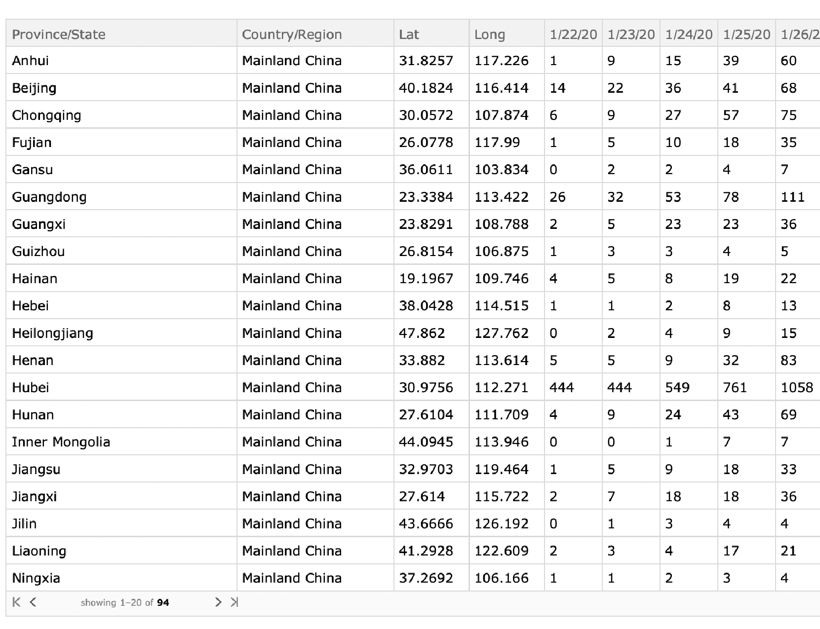
confirmed=Import["https://raw.githubusercontent.com/CSSEGISandData/COVID-19/master/csse_covid_19_data/csse_covid_19_time_series/time_series_19-covid-Confirmed.csv"];confirmed[[1]][[-1]]
Out[]=
2/25/20
South Korea
South Korea
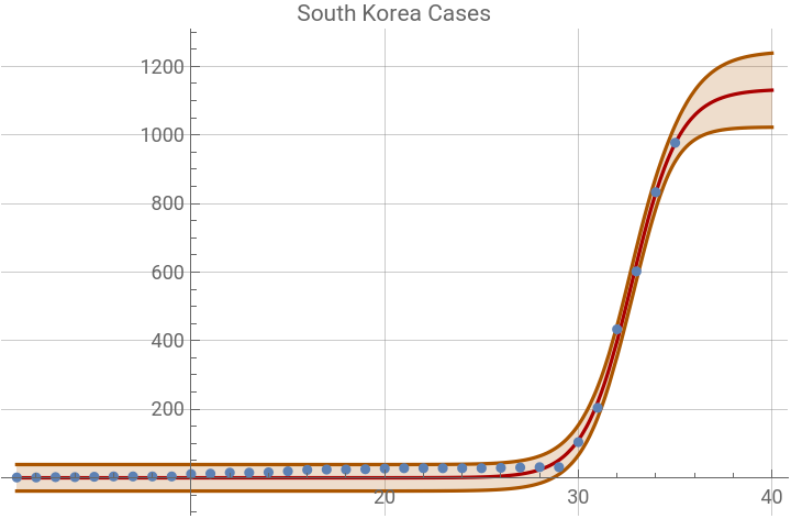
I suspect that the flat growth up to day 29 shows a small group of infected and exposed people successfully quarantined. Suddenly on day 30 there is a new outbreak, probably from an unknown source who wasn’t tracked with the initial group.
In[]:=
ListPlot[Tooltip/@skoreaCases0,PlotRangeAll]
Out[]=
In[]:=
skoreaNLM=NonlinearModelFit[skoreaCases,logistic,{{k,0.3},{L,2000},{t0,50}},t];skoreaNLM["BestFitParameters"]
Out[]=
{k0.809863,L1133.63,t032.7558}
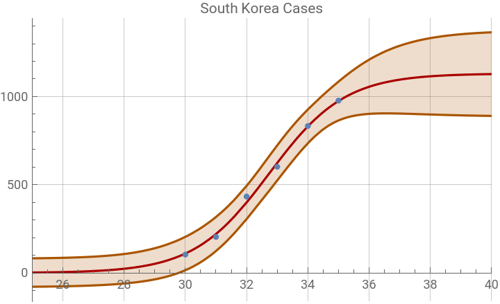
The fits are surprisingly similar even when most of the initial points are dropped. This an interesting result of accumulated data -- all of the information is packed into the most recent points. It only takes three accurate points to fit the whole logistic curve.
In[]:=
skoreaNLM1=NonlinearModelFit[Drop[skoreaCases,29],logistic,{{k,0.3},{L,2000},{t0,50}},t];skoreaNLM1["BestFitParameters"]
Out[]=
{k0.812442,L1130.48,t032.7449}
The fits with 95% confidence intervals.
Out[]=
Out[]=
In[]:=
skoreaNLM@"ParameterConfidenceIntervalTable"skoreaNLM1@"ParameterConfidenceIntervalTable"
Out[]=
Estimate | Standard Error | Confidence Interval | |
k | 0.809863 | 0.0539538 | {0.699963,0.919764} |
L | 1133.63 | 51.1127 | {1029.52,1237.74} |
t0 | 32.7558 | 0.152211 | {32.4458,33.0659} |
Out[]=
Estimate | Standard Error | Confidence Interval | |
k | 0.812442 | 0.0818155 | {0.552069,1.07282} |
L | 1130.48 | 72.3516 | {900.223,1360.73} |
t0 | 32.7449 | 0.212604 | {32.0683,33.4215} |
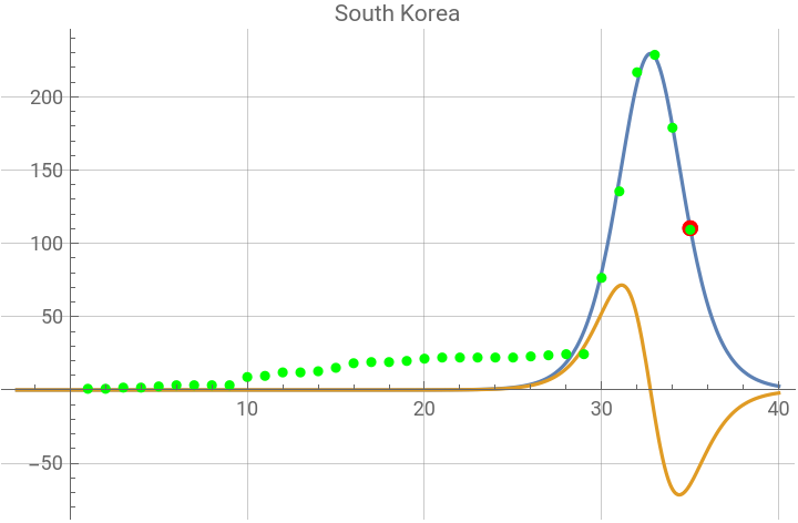
This graphic shows the first and second derivative plots of the logistic function. The red dot is at the current day number on the first derivative curve. The green dots are the points calculated by the logistic differential equation, using each data point. The prediction for the last case date is printed (probably not accurate until there are at least three weeks of new data).
Last case: Tue 3 Mar 2020
Out[]=


Italy
Italy
The model doesn’t support an accumulated case number of 0, which occurs at t -∞. Also the initial cases probably didn’t increase for a number of days, because they were isolated were not likely responsible for the outbreak. So we begin italyCases at day 31 as a new outbreak.
2/25/20
It is too soon after the recent infection spike to accurately calculate k, which is much higher than for China with the limited data. The logistic function with the higher k than observed in China, shows a relatively early termination, which will probably be unlikely as more data becomes available.
It is too soon after the recent infection spike to accurately calculate k, which is much higher than for China with the limited data. The logistic function with the higher k than observed in China, shows a relatively early termination, which will probably be unlikely as more data becomes available.
Below, an initial exploration of method to fit data directly to differential equation of the logistic function.
Each point difference is a linear expression
This version solves for the first derivative of the interpolation = 0.