The problem we discuss here is modeling spin network interactions via branchial graphs of MultiwaySystems. A spin network can be thought of as an extension of the Ising model in which the material is a 1D or 2D lattice with a spin doublet associated with each site inside the lattice. The doublet of each site indicates that spin direction is either up or down for that specific site. Often, spin-spin interactions can only happen between the nearest neighbors. In the case we are interested in, each site can interact with further sites as well and the interactions between different sites can be encoded in hypergraph edges connecting corresponding nodes inside the graph. Hence, the Hamiltonian of the system can be extracted from connectivity of the branchial graphs. Having the Hamiltonian, one can compute energy of the system in any state, its partition function, the free energy or entropy.
Theory
Theory
The Ising model describes spin-spin interaction between a number of sites inside a material. Originally, the interactions is restricted only to the nearest neighbors. For a given spin configuration {} for the whole lattice and in the presence of an external magnetic field , the energy of the system is given by
S
i
B
i
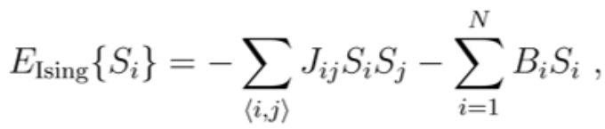
where <i,j> indicates that only nearest neighbors interact, i.e. j=i±1. The model first proposed to describe the ferromagnetic behaviour for >0. Later, anti-ferromagnetism was also explained by the same model for <0. Having the energy of each configuration, one can obtain the partition function of the system by taking into account all possible spin configurations, i.e.
J
J

Multiway Systems & Branchial Graphs
Multiway Systems & Branchial Graphs
The main idea is to generate spin networks containing more complex interactions between sites. There are two main motivation for choosing Multiway systems for this purpose:
◼
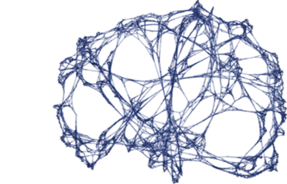
Given the replacement rules, Multiway systems can generate absolutely non-trivial graphs.
◼
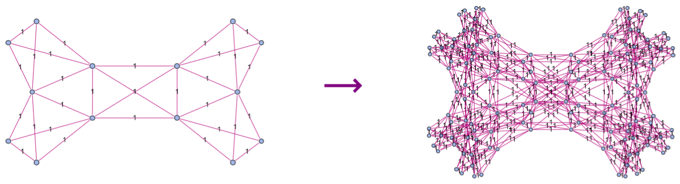
Time evolution of the physical system is captured by higher generation of the branchial graphs.
1. Framework
1. Framework
For simplicity, here we do not consider interaction with an external magnetic field (=0). To proceed, we first need to define the spin operator “” for each site. Given the fact that “” always takes integer and half-integer values, we first impose the following condition
B
i
s
z
s
In[]:=
SpinQ[S_]:=IntegerQ[2S]&&S>=0
and then define
In[]:=
sz[S_?SpinQ]:=sz[S]=SparseArray[Band[{1,1}]->Range[S,-S,-1],{2S+1,2S+1}]id[S_?SpinQ]:=id[S]=IdentityMatrix[2S+1,SparseArray]
Now we need to extend the spin operator so that every time it acts on th site as spin operator while its action on all other sites is trivial. Mathematically speaking, for a (2+1)×(2+1) matrix associated to the site
k
S
S
A
k

where is the number of sites inside the network. For our purpose the operator will simply be and that can be done via
N
A
s
z
Spinop[S_?SpinQ,n_Integer,k_Integer,sz_?MatrixQ]/;1<=k<=n&&Dimensions[sz]=={2S+1,2S+1}:=KroneckerProduct[IdentityMatrix[(2S+1)^(k-1),SparseArray],sz,IdentityMatrix[(2S+1)^(n-k),SparseArray]]sz[S_?SpinQ,n_Integer,k_Integer]/;1<=k<=n:=Spinop[S,n,k,sz[S]]
There is also an matrix whose elements physically determine the coupling coefficients between various sites/nodes inside the network. If we restrict the interactions only to the nearest neighbor as we do for the original Ising model, the matrix take the following form
N×N
J
In[]:=
JIsing[n_Integer,k_Integer]:=Array[Subscript[J,#1,#2]&,{n,n}][[k,Mod[k+1,n,1]]]
Given , the Hamiltonian for spin-spin interaction will become
J
In[]:=
HIsing[S_?SpinQ,n_Integer/;n>=3]:=-Sum[J[n,k]*sz[S,n,k].sz[S,n,Mod[k+1,n,1]],{k,n}]
In our case, the matrix is something to be obtained from a graph generated by the Multiway systems. First thing to do is generating a generally non-trivial graph where each node presents a spin site inside the network. To do so, we need to determine a replacement rule along with an initial state to start with. Then we focus on a branchial graph of a specific generation. A 1D spin chain is then generated by
J
In[]:=
Chain[rule_,init_,gen_Integer]:=ResourceFunction["MultiwaySystem"][rule,init,gen,"BranchialGraphStructure",EdgeLabels->"EdgeWeight"]
where the connectivity of the generated graph is encoded by its adjacency matrix
In[]:=
AChain[Chain_]:=Normal[AdjacencyMatrix[Chain]]
using which, one can introduce a weighted coupling matrix “”between various sites
a
amat[n_]:=Table[Subscript[a,i,j],{i,n},{j,n}]a[AChain_,amat_,n_]:=Table[If[AChain[[i,j]]==0,0,amat[[i,j]]],{i,n},{j,n}]
Depending on the model under study, one might be rather interested in a symmetric coupling matrix
In[]:=
aSym[n_,a_]:=Table[If[i>j,a[[j,i]],a[[i,j]]],{i,n},{j,n}]
However, there exist models in which the coupling matrix is not necessarily symmetric. Finally, we obtain the Hamiltonian of the system
In[]:=
H[S_?SpinQ,a_,n_Integer/;n>=3]:=-SparseArray[Sum[a[[i,j]]*sz[S,n,i].sz[S,n,j],{i,n},{j,n}]]
Now, we pick up a random spin state for each site and then take the direct product of states over all sites to determine the spin configuration for the whole network
ranspin[n_Integer]:=RandomChoice[{{{1},{0}},{{0},{1}}},n]Spinst[ranspin_]:=KroneckerProduct@@ranspin
Putting all together, one can now calculate the energy of the system for a specific spin configuration.
Now, let us explicitly apply this framework for two examples.
Now, let us explicitly apply this framework for two examples.
2. Examples
2. Examples
2.1 Ex.1: Ising Model
2.1 Ex.1: Ising Model
We start with a spin chain with only neighbors interacting
In[]:=
ChainIs=Chain["A"->"AB","AA",4]
Out[]=

To check the way nodes are connected
AChainIs=AChain[ChainIs];amatIs=amat[5];aIs=a[AChainIs,amatIs,5];aIsSym=aSym[5,aIs];ranspinIs=ranspin[5];SpinstIs=Spinst[ranspinIs];HIs=Simplify[H[1/2,aIsSym,5]];
In[]:=
EnergyIs=Sum[Transpose[SpinstIs[[i]]]HIs[[i,j]]SpinstIs[[j]],{i,32},{j,32}]
Out[]=
+++
a
1,2
2
a
2,3
2
a
3,4
2
a
4,5
2
2.2 Ex2.: A Chaotic Network
2.2 Ex2.: A Chaotic Network
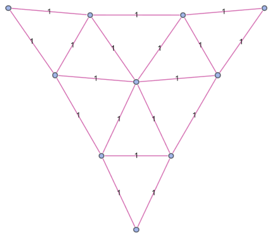
Let us consider a rather chaotic network in which each site might be coupled to a number of further sites. This time the network is generated by a different replacement rule and a new initial state. Pursuing the same procedure, we will have
In[]:=
Net=Chain["A"->"BA","AAA",3]
Out[]=
ANet=AChain[Net];amatNet=amat[10];aNet=a[ANet,amatNet,10];HNet=Simplify[H[1/2,aNet,10]];ranspinNet=ranspin[10];SpinstNet=Spinst[ranspinNet];
which for a symmetric spin interaction will reduces to
Results & Possible extensions
Results & Possible extensions
◼
The Hamiltonian operator is constructed for an arbitrary spin network with more general interaction than the original Ising model.
◼
The energy of the network in a specific spin configuration is calculated.
◼
As one might noticed, the replacement rule we apply for the Multiway system is crucial as it basically determines the topology of the graph and the way various nodes are connected. Hence, it is interesting to trace its possible effects on the final partition function.
◼
To go beyond the original Ising model, the next thing that cross the mind is to couple each site to its next to nearest neighbor as well. That would describe the higher order behavior of a spin network. To do so, one first need to find the proper replacement rule for the Multiway system that generates a spin network with this type of higher order couplings. However, this seems a nontrivial task to do.
◼
The study can be extended to various systems of particles with more complex interactions. For instance, adding other physical features such as mass and electromagnetic charge one can study the behaviour of a gas of charged particles and look for the relevant physical quantities.
◼
In Multiway systems, the time evolution of the system translates to looking at the Multiway graphs of higher generations. So here one can also study the time evolution of relevant physical quantities and their expectation values.