Find first part here: https://community.wolfram.com/groups/-/m/t/3340354
Abstract: The Schrödinger equation is central to quantum mechanics, describing the time evolution of wavefunctions in both analytical and numerical contexts. Bohmian mechanics extends this framework by providing a causal interpretation of quantum phenomena, linking the wavefunction to particle trajectories through the gradient of its phase or the quantum potential. This paper explores Fourier analysis as a fundamental tool for solving the Schrödinger equation, enabling transitions between momentum and position space to simplify differential equations. Part 1 introduces continuous Fourier methods, while Part 2 focuses on numerical solutions using the discrete Fourier transform (DFT). The DFT is particularly valuable in simulations, replacing computationally intensive numerical differentiation with efficient algebraic operations. Applications include one-, two-, and three-dimensional systems, emphasizing wavefunction superposition, interference, and particle scattering at potentials. Mathematica is employed as the computational framework for this investigation, leveraging its advanced Fourier capabilities to examine Bohmian trajectories and optimize wavefunction calculations.
Full list of posts: https://community.wolfram.com/web/kvbloh/
Note: see the detailed introduction to the de Broglie Bohm theory and implicit scheme method here:
https://community.wolfram.com/groups/-/m/t/3000266
https://community.wolfram.com/groups/-/m/t/3143785
https://community.wolfram.com/groups/-/m/t/3145353
https://community.wolfram.com/groups/-/m/t/3240209
5. Numerical Methods
5. Numerical Methods
Numerical methods [2, 4, 5, 7, 8] are indispensable for the solution of quantum mechanical problems, especially when analytical solutions are not available. Among these, the Discrete Fourier Transform (DFT) emerges as a powerful and efficient technique for computing wavefunctions in quantum systems [5, 8]. The DFT is particularly advantageous for solving the time-dependent Schrödinger equation, as it enables seamless transitions between position and momentum spaces, significantly simplifying the numerical treatment of differential operators like the kinetic energy term.
Specifically, the DFT converts a discretized function from its original domain—typically position space—into momentum space, where differential operations such as the Laplacian operator are transformed into simpler algebraic operations. In position space, the Laplacian involves computationally intensive second-order derivatives, but in momentum space, it simplifies to a straightforward multiplication by a factor proportional to the square of the momentum components. This transformation not only reduces computational complexity but also enhances the efficiency and accuracy of time-dependent quantum mechanical simulations. The methods implemented here are grounded in well-established algorithms, as detailed in [2]. Below you will find a small selection of original titles from the first publications and current books.
Specifically, the DFT converts a discretized function from its original domain—typically position space—into momentum space, where differential operations such as the Laplacian operator are transformed into simpler algebraic operations. In position space, the Laplacian involves computationally intensive second-order derivatives, but in momentum space, it simplifies to a straightforward multiplication by a factor proportional to the square of the momentum components. This transformation not only reduces computational complexity but also enhances the efficiency and accuracy of time-dependent quantum mechanical simulations. The methods implemented here are grounded in well-established algorithms, as detailed in [2]. Below you will find a small selection of original titles from the first publications and current books.
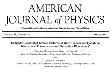
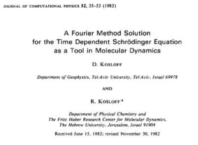
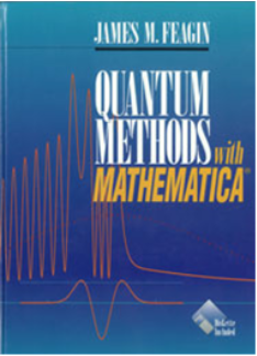

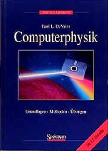
Figure 4. Original titles
5.1 The Discrete Fourier Transform (DFT)
5.1 The Discrete Fourier Transform (DFT)
In the discrete Fourier method, spatial (configuration) space and time are discretized with a uniform grid, whereby the discrete Fourier transform (DFT) of the discrete wave function, for a timestep can be written as: ()Ψ() , where () is the wavefunction in momentum (or wavenumber) space, is the discrete wave number, NP is the number of spatial grid points and are the discrete position values. The inverse Discrete Fourier Transform (iDFT), which retrieves the wavefunction in configuration space from its momentum representation, is given by: .Although emphasised earlier, it should be reiterated that the DFT facilitates the transitions between space and momentum representations of the wave function and simplifies the numerical treatment of the Schrödinger equation. By transforming the Laplacian operator from a computationally intensive second derivative in position space to a simple multiplication in momentum space, DFT increases efficiency. In momentum space, the second derivative becomes a multiplication operation Ψ()-(). An inverse Fourier transformation leads back to the wave function in the spatial space. The potential energy, which remains a function of position, is applied in configuration space. Therefore, an alternating series of Fourier transforms between position and momentum (or wavenumber) spaces is typically used to apply the Hamiltonian in a step-by-step process, often referred to as the split-operator method. Thus, a combination of DFT and inverse iDFT operations is employed to efficiently evolve the wavefunction in time. To ensure stability and accuracy in the numerical solution of the time-dependent Schrödinger equation using the discrete Fourier transform, the time step and the spatial grid spacing must be carefully matched [6]. A smaller grid spacing increases the resolution in the spatial domain, but also requires smaller time steps in order to maintain stability - this results from the so-called CFL condition [20]. The following algorithms use and , which are suitable in most cases.The DFT and inverse iDFT operations can be easily realised with the Mathematica ‘built-In’ functions ‘Fourier’ and ‘InverseFourier’, but they set the grid origin of their argument list to the left end of the grid, i.e. to the first element of the argument list. This must be taken into account in the solution. The grid required for the solution grid must be set up with the origins in the centre of the grid and number of grid points must be odd for the correct overall phase function. It is therefore necessary to shift or rotate the grid wave function by half a grid length. This can be done with the Mathematica ‘built-In’ function ‘Rotate’ or the command ‘ResourceFunction[’FourtierShift‘]’ and shifting the list one position to the right.
Ψ(,)
x
n
t
n
t
n
Ψ
x
n
t
n
Ψ
k
n
NP
∑
n0
x
n
-2iπ
k
n
NP
e
Ψ
k
n
k
n
x
n
Ψ()()
x
n
1
NP
NP
∑
n0
Ψ
k
n
2π i
x
n
NP
e
2
∂
x
n
∂
2
x
2
k
ψ
k
n
Δt
Δx
Δx
Δt
δ≈
T
2NP
ϵ
L
NP
Note: The transformation between ‘world coordinates’ and ‘screen coordinates’ is a fundamental concept in computational graphics, enabling the representation of abstract data in a format suitable for display on a two-dimensional screen. World coordinates define a spatially accurate and often device-independent system, while screen coordinates map this representation to the pixel grid of a display device, ensuring compatibility with visualization requirements. In this paper, for the sake of clarity and ease of implementation, a reverse transformation back to world coordinates has been omitted in most of the cases. This approach simplifies the process of making modifications to the underlying code listings, as screen coordinates directly correlate with the visual output and allow for more intuitive adjustments.
5.2 Solving the Schrödinger Equation with the DFT and the Split Operator Method
5.2 Solving the Schrödinger Equation with the DFT and the Split Operator Method
To solve the time-dependent Schrödinger equation numerically, the wavefunction is first discretized on a grid in real space. The time evolution of the wavefunction can be performed using several methods such as the Crank-Nicolson method or the split-operator method [4, 7]. The key steps in using the DFT approach are as follows [2, 5]:
Discretization of the Wavefunction: The position space is divided into a grid of points, and the wavefunction is evaluated at each grid point. The DFT is then applied to transform this discrete wavefunction into momentum space.
Shifting the Lattice: Shifting the wave function by half a grid length enables the overall phase function to be calculated correctly. The symmetrical arrangement of the frequencies maintains the symmetry between the phase function and the wave function.
Kinetic Energy Term: In momentum space, the kinetic energy operator becomes a simple multiplication, which significantly reduces computation time.
Potential Energy Term: The potential energy operator is applied in configuration space. After calculating the kinetic energy term in momentum space, the inverse DFT is used to return the wavefunction to configuration space, where the potential is applied.
Time Propagation: The time evolution of the wavefunction is typically handled using methods such as the Crank-Nicolson method or the split-operator method. These methods break the Hamiltonian into kinetic and potential parts. The DFT is used to alternate between momentum and spatial (Configuration) space at each time step, enabling efficient application of both terms.
Discretization of the Wavefunction: The position space is divided into a
NP
Shifting the Lattice: Shifting the wave function by half a grid length enables the overall phase function to be calculated correctly. The symmetrical arrangement of the frequencies maintains the symmetry between the phase function and the wave function.
Kinetic Energy Term: In momentum space, the kinetic energy operator becomes a simple multiplication, which significantly reduces computation time.
Potential Energy Term: The potential energy operator is applied in configuration space. After calculating the kinetic energy term in momentum space, the inverse DFT is used to return the wavefunction to configuration space, where the potential is applied.
Time Propagation: The time evolution of the wavefunction is typically handled using methods such as the Crank-Nicolson method or the split-operator method. These methods break the Hamiltonian into kinetic and potential parts. The DFT is used to alternate between momentum and spatial (Configuration) space at each time step, enabling efficient application of both terms.
There are several limitations associated with this approach. Firstly, in the discrete Fourier transform (DFT), periodic boundary conditions are inherently assumed, meaning the values at the boundaries of the spatial grid are treated as if they repeat continuously. This implies that the function, such as a wavefunction, wraps around seamlessly from one end of the grid to the other, creating a closed loop where the left and right boundaries are effectively connected. So, Incorrect boundary conditions can lead to artefacts in the solution. To minimize this, careful design of the grid and boundaries is required.
Secondly, the accuracy of the DFT depends on the the spatial grid points. A higher number of grid points leads to a better resolution, but at the cost of a higher computational effort. Similarly, the time step used in the temporal evolution must be carefully chosen to ensure stability and accuracy. The Crank Nicolson method is used for comparison to ensure the accuracy of the algorithm and the certainty of the physical significance.
Secondly, the accuracy of the DFT depends on the the spatial grid points. A higher number of grid points leads to a better resolution, but at the cost of a higher computational effort. Similarly, the time step used in the temporal evolution must be carefully chosen to ensure stability and accuracy. The Crank Nicolson method is used for comparison to ensure the accuracy of the algorithm and the certainty of the physical significance.
Note: Arrangement of Shifting the Lattice:
In the numerical simulation, the discrete Fourier transform (DFT) assumes that the origin of the lattice is at the ‘left’ end of the lattice and starts at zero. In the quantum systems used with centred wave functions, the potential is initialized symmetrically around the centre of the lattice. This leads to asymmetric phase components and inconsistencies in the trajectories (asymmetric trajectories) if they are not corrected. By shifting the wave function by half a grid length, the centred wave function is adapted to the structure of the DFT based on the origin. This adjustment ensures that the zero wavenumber component is correctly positioned in the centre of the wavenumber spectrum when using the fast Fourier transform (FFT) and that the phase symmetry is maintained. In order to maintain the symmetry of the overall phase function, it is necessary here that the number of grid points is odd. There are three ways to include the shift of the zero frequency term to the centre of the spectrum in the algorithm.
Please note that for the correct results of methods 2 and 3 it is necessary to shift the list one position to the right. Although in this case the list is shifted asymmetrically around the zero point, the wave function itself remains symmetric and shows precise agreement with the Crank-Nicolson method (to be honest I don’t know why). The functions for methods 2 and 3 come from Mathematica ResourceFunction and from the Mathematica stack Exchange:
In[]:=
ResourceFunction["FourierShift"]
Out[]=
In[]:=
fftshift[dat_?ArrayQ,k:(_Integer?Positive|All):All]:=Module[{dims=Dimensions[dat]},RotateRight[dat,If[k===All,Quotient[dims,2],Quotient[dims[[k]],2]UnitVector[Length[dims],k]]]];
In[]:=
NP=5;kzmax=4;Print["Unshifted:"]Kinetic=Array[#&,NP,{0,kzmax}]//NPrint["Method 1: Shifted:"]Kinetic1=Array[#&,NP,{0,kzmax}]//RotateLeft[#,(NP-1)/2]&//NPrint["Method 2: Shifted:"]Kinetic2=ResourceFunction["FourierShift"][Array[#&,NP,{0,kzmax}]]//RotateRight[#,1]&//NPrint["Method 3: Shifted:"]Kinetic3=fftshift[Array[#&,NP,{0,kzmax}]]//RotateRight[#,1]&//N
Unshifted:
Out[]=
{0.,1.,2.,3.,4.}
Method 1: Shifted:
Out[]=
{2.,3.,4.,0.,1.}
Method 2: Shifted:
Out[]=
{2.,3.,4.,0.,1.}
Method 3: Shifted:
Out[]=
{2.,3.,4.,0.,1.}
5.3 The Double-Well Potential
5.3 The Double-Well Potential
The double well potential is used here to apply the DFT method. The double-well potential is a fundamental model in quantum mechanics that describes the motion of a particle in a space with two potential minima separated by a barrier [12]. It describes the potential energy to which a quantum mechanical particle is subjected in a specific space, where two separate potential minima exist, separated by a barrier. Such a system is often used to study the quantum phenomena of tunneling and oscillation. Classically, a particle would remain trapped in one of these minima, because its kinetic energy is insufficient to overcome the barrier. This aligns with the everyday understanding of physical systems where particles reside in stable states. But according to quantum mechanics, it can oscillate between the two minima by tunneling through the barrier. According to the principles of quantum mechanics, the particle is not confined to these minima. It can overcome the barrier through a quantum mechanical phenomenon called tunneling and oscillate between the two minima. The double well potential is defined by with the box length and ,L,a,b∈. In this specific potential, the minima of the potential are located at , and the barrier reaches a height of at .
V=-L
V
max
2
1
L
2
(x-a)
2
b
L
V
max
x=a±bL
V=
4
b
2
L
V
max
x=a
In[]:=
Clear[Vmax,L,a,b]Vpot[x_]=Vmax(1/L(x-a)^2-L*b^2)^2;Print["Extreme values: "]sol=Solve[D[Vpot[x],x]==0,x]Print["Maximum: "]Vpot[x]/.sol[[1]]
Extreme values:
Out[]=
{{xa},{xa-bL},{xa+bL}}
Maximum:
Out[]=
4
b
2
L
The next plot show the potential.
In[]:=
Manipulate[Plot[Vmax(1/L(x-a)^2-L*b)^2,{x,-10,10}],{{L,20},1,40,Appearance"Labeled"},{Vmax,1,2,0.2,Appearance"Labeled"},{{a,0},-2,2,0.2,Appearance"Labeled"},{{b,0.1},0.1,1.0,0.02,Appearance"Labeled"}]
Out[]=


5.4 The Discrete Fourier Transform with the Split - Operator Method
5.4 The Discrete Fourier Transform with the Split - Operator Method
6. The Causal Interpretation of Quantum Mechanics
6. The Causal Interpretation of Quantum Mechanics
6.1 Numerical Computation of the Quantum Potential (QP)
6.1 Numerical Computation of the Quantum Potential (QP)
In the graph you can see the wave density and the quantum potential, the quantum potential and the potential are scaled and sometimes have to be adjusted for the graphical representation.
6.2 Numerical Computation of Trajectories
6.2 Numerical Computation of Trajectories
It is important to emphasise that the parameters must be chosen carefully in order to generate a physically meaningful simulation. The graph shows the density of the wavefunction, the quantum potential and the one-dimensional velocity field. Artefacts occur at the edges of the lattice in the quantum potential and especially in the velocity field. For this reason, the velocity field is only displayed within the potential. For large potential values, you can clearly see that the wave density is reflected at the edge of the potential. If the barrier between the minima within the potential is small, the interference between the two wave packets is largely retained. For longer periods, interference effects and reflection effects overlap, resulting in interesting wave patterns. Please just try it out.
In certain cases (high oscillation), this can increase the calculation time. In our case, the oscillation had no major great influence on the calculation time. Due to the numerical error the velocity term must be adjusted sometimes.
The graphic on the right shows the squared wavefunction, the potential, and the trajectories. The graphic on the left shows the particles’ positions, the squared wavefunction (red), the quantum potential (blue) and the potential (black). The representation of the wave density and the potentials are scaled and sometimes have to be adjusted.
IMPORTANT: Performance Warning
The creation of the ‘video frames’ can be very time-consuming due to the CPU capacity. It is recommended that you use the results specified at the beginning of the section. Save the results that you have created up to this point.
IMPORTANT: Performance Warning
The creation of the ‘video frames’ can be very time-consuming due to the CPU capacity. It is recommended that you use the results specified at the beginning of the section. Save the results that you have created up to this point.
7. Comparing Two Methods
7. Comparing Two Methods
The next step is to determine the quantum potentials for the two methods used.
IMPORTANT: Performance Warning
The calculations can be time-consuming due to the CPU capacity.
IMPORTANT: Performance Warning
The calculations can be time-consuming due to the CPU capacity.
Significant deviations can be recognised between the two methods, which are due to the artefact that in the Crank Nicolson method (CN) the wavefunction is reflected at the edges of the box and therefore the shape of the wave changes over time. In contrast, the Fourier method applies periodic boundary conditions, meaning the wave function smoothly continues from the left edge of the grid to the right, creating a seamless loop. These effects disappear for the wavefunction if the wave remains within the potential or if the box length is increased or the wave number is reduced. Then, the same results are then obtained without significant deviations for the quantum potential and wavefunction. However, the huge advantage lies in the time comparison. The Discrete Fourier Transform method (DFT) is (depending on the hardware used) many times faster than the Crank-Nicolson method (without time-reducing algorithms within the CN method).
8. The Two-Dimensional Treatment of the Schrodinger Equation with the DFT
8. The Two-Dimensional Treatment of the Schrodinger Equation with the DFT
IMPORTANT: Performance Warning
The calculations and the creation of the ‘video frames’ can be very time-consuming due to the CPU capacity. It is recommended that you use the results specified at the beginning of the chapter. Save the results that you have created up to this point.
The calculations and the creation of the ‘video frames’ can be very time-consuming due to the CPU capacity. It is recommended that you use the results specified at the beginning of the chapter. Save the results that you have created up to this point.
8.1 The Calculation of the Trajectories
8.1 The Calculation of the Trajectories
In the graphic above, one can observe the density of the wavefunction as well as the possible trajectories and the potential (red, if enabled) depending on the initial points.
8.1.2 Enhanced Visualization of Quantum Dynamics through 3D Representation
8.1.2 Enhanced Visualization of Quantum Dynamics through 3D Representation
Under the influence of a potential, the wave function typically exhibits interference patterns and scattering effects( in the graph above, no potential is used). As the potential height decreases, tunneling processes become visible: a lower potential reduces the barrier encountered by the wave function, increasing the probability of penetrating the potential barrier. This results in a noticeable increase in wave function transmission through the potential region, often observed as an elevated wave density on the opposite side of the potential barrier. In summary, it can be said that in Bohmian mechanics these processes are described in more detail by particle trajectories that follow the phase of the wave function. They thus enable a better understanding of the behaviour of particles in regions inside and outside the potential.
9. The Three-Dimensional Treatment of the Schrodinger Equation with the DFT
9. The Three-Dimensional Treatment of the Schrodinger Equation with the DFT
As an extension of the previously presented implementations of the discrete Fourier transform for one- and two-dimensional systems, the three-dimensional DFT requires only a few specific adjustments to calculate the wavefunction. The extension to three-dimensional space enables a more comprehensive analysis of systems with more complex potential structures and allows detailed and more intuitive investigations of spatial interactions and quantum mechanical effects that are only visible to a limited extent in lower dimensions. However, it should be noted that the computing time increases, which leads to a limited utilisation of grid points.
9.1 Exploring Elliptical - Cylindrical Potentials
9.1 Exploring Elliptical - Cylindrical Potentials
The potential under consideration has a cylindrical shape and is aligned perpendicular to the direction of propagation of the wave packet. In contrast to a circular cross-section, this potential has an elliptical cross-section, which disturbs the rotational symmetry along the axes parallel to the movement of the wave packet. This elliptical-cylindrical shape alters the scattering and interference patterns by imposing directional constraints on the wave packet as it traverses the potential. As a result, the calculations of the trajectories and the wave function density reflect the different influences of the elliptical confinement. To investigate these interference effects and scattering effects, two wave packets with wavenumbers that differ only in sign are directed to the potential. If you change the grid points, the data for the positioning and dimensioning of the potential may need to be adjusted.
IMPORTANT: Performance Warning
The calculations and the creation of the ‘video frames’ can be very time-consuming due to the CPU capacity. It is recommended that you use the results specified at the beginning of the chapter. Save the results that you have created up to this point.
The calculations and the creation of the ‘video frames’ can be very time-consuming due to the CPU capacity. It is recommended that you use the results specified at the beginning of the chapter. Save the results that you have created up to this point.
The graph above shows the wave density and the potential. Please note that the x and z values are reversed. This must be taken into account when determining the velocity terms. If you change the grid points, the data for initial positions may need to be adjusted.
The diagram above only shows the possible paths depending on the starting positions.
The graph above shows the wave density, the possible paths and the potential.
Notes: During editing, the screen coordinates simplify visual adjustments as they relate directly to the display parameters. If the number of grid points is increased, the distance for the starting positions of the tracks must also be adjusted. With the number of grid points used, the distances for the trajectories were set to 6 and 4 screen points. For the video animation, ‘world coordinates’ are applied to present the simulation in its correct spatial relationship and independently of screen resolution, which used in the previous animation. Depending on the hardware, the computing time is approx. 400 seconds.
Notes: During editing, the screen coordinates simplify visual adjustments as they relate directly to the display parameters. If the number of grid points is increased, the distance for the starting positions of the tracks must also be adjusted. With the number of grid points used, the distances for the trajectories were set to 6 and 4 screen points. For the video animation, ‘world coordinates’ are applied to present the simulation in its correct spatial relationship and independently of screen resolution, which used in the previous animation. Depending on the hardware, the computing time is approx. 400 seconds.
References
References
A heartfelt thank you to the Wolfram Team for their invaluable support in developing my programs with Mathematica. I am especially grateful to Vitaliy Kaurov and Ahmed Elbanna for their expert guidance and patience throughout the entire project.
A selection of animations can be seen in some of the author’s videos (Other Internet Sources: [1-6]).
A selection of animations can be seen in some of the author’s videos (Other Internet Sources: [1-6]).
Wolfram Demonstrations by Klaus von Bloh and Vikram Athalye
Wolfram Demonstrations by Klaus von Bloh and Vikram Athalye
Wolfram Demonstrations by Klaus von Bloh
Wolfram Demonstrations by Klaus von Bloh
Wolfram Community posts by Klaus von Bloh
Wolfram Community posts by Klaus von Bloh
Articles
Articles
[1] C. G. Darwin, “Free motion in the wave mechanics,” Proceedings of the Royal Society A, 117, 1927 pp. 258–293 . /doi.org/10.1098/rspa.1927.0179.
[2] J. M. Feagin, Quantum Methods with Mathematica, New York, TELOS/Springer-Verlag, 1994.
[3] R . W . Robinett,”Quantum wave packet revivals,” Physics Repo rts, 392(1–2), 2004 pp. 1-119. doi.org/10.1016/j.physrep.2003.11.002. arXiv:quant-ph/0401031.
[4] A. Goldberg, H. Schey, and J. L. Schwartz, “Computer-Generated Motion Pictures of One-Dimensional Quantum Mechanical Transmission and Reflection Phenomena,” American Journal of Physics., 35(3), 1967 pp. 177–186.
[5] D. Kosloff and R Kosloff Abraham, “A fourier method solution for the time dependent Schrödinger equation as a tool in molecular dynamics,” Journal of Computational Physics, 52(1), 1983 pp. 35–53. doi: 10.1016/0021-9991(83)90015-3.
[6] R. D. Richtmyer and K. W. Morton, Difference Methods for Initial-Value Problems, New York,John Wiley & sons, 1967.
[7] B. Thaller, Visual Quantum Mechanics, New York: Springer-TELOS, 2000.
[8] P. L. DeVries, Computerphysik, Heidelberg: Spektrum Akademischer Verlag , 1995.
[9a] C. Dewdney and B. J. Hiley, “A Quantum Potential Description of One-Dimensional Time-Dependent Scattering from Square Barriers and Square Wells,” Foundations of Physics 12(1), 1982 pp. 27–48. doi: 10.1007/BF00726873.
[9b] C. Philippidis, C. Dewdney and B. J. Hiley, “Quantum Interference and the Quantum Potential,” Il Nuovo Cimento B Series 11, 52(1), 1979 pp. 15–28. doi:10.1007/BF02743566.
[10a] D. Bohm, “A suggested Interpretation of the Quantum Theory in Terms of Hidden Variables, I,” Physical Review 85 (2), 1952 pp. 166–179. doi:10.1103/PhysRev.85.166.
[10b] D. Bohm, “A suggested Interpretation of the Quantum Theory in Terms of Hidden Variables, II,” Physical Review 85 (2), 1952 pp. 180–193. doi:10.1103/PhysRev.85.18.
[11] P . R . Holland, The Quantum Theory of Motion: An Account of the de Broglie–Bohm Causal Interpretation of Quantum Mechanics, New York : Cambridge University Press, 1993.
[12] [1] P. Ghose, Y. Mirgorod, “Relationship between classical and quantum mechanics in micellar aqueous solutions of surfactants,” Physics of Wave Phenomena 32, 2024 pp 34–42. doi:10.3103/S1541308X24010072 or arxiv:2306.06618v1 [quant-ph].
[13] P. Ghose and K. von Bloh, “Continuous Transitions between Quantum and Classical Motions,” arxiv:1608.07963v2 [quant-ph].
[14] S. Goldstein. “Bohmian Mechanics.” The Stanford Encyclopedia of Philosophy. (Oct 8, 2024) plato.stanford.edu/entries/qm-bohm.
[16] D.Bohm and J.P. Vigier, “Model of the Causal Interpretation of Quantum Theory in Terms of a Fluid with Irregular Fluctuations,” Physical Review 96(20), 1954 pp. 208–216. doi:10.1103/PhysRev.96.208.
[18] Wikipedia. “ Configuration space.” (Jul 4, 2024) https://en.wikipedia.org/wiki/Configuration_space_(physics).
[20] Wikipedia. “Courant–Friedrichs–Lewy condition.” (Jul 4, 2024) https://en.wikipedia.org/wiki/Courant%E2%80%93Friedrichs%E2%80%93Lewy_condition.
[23] Wikipedia. “Fourier transform.” (Nov 24, 2024) https://en.wikipedia.org/wiki/Fourier_transform.
Other Demonstrations and internet sources
Other Demonstrations and internet sources
[1] Paul Nylander (see also his homepage) and E. Zeleny, “Probability Density for an Electron Passing through Two Narrow Slits”, Wolfram Demonstrations Project, 2012.
[2] Paul Nylander (see also his homepage) and E. Zeleny, “Probability Density Distribution for Electron Scattering”, Wolfram Demonstrations Project, 2012.
[3] K. Das, “Fraunhofer Diffraction at a Single Slit”, Wolfram Demonstrations Project. Wolfram Demonstrations Project, 2016.
Other Internet Sources:
[1] K. von Bloh.Quantum Motion in an Elliptical Smooth Potential with a Repelling Coulomb-like Potential [Video]. (Oct 28, 2024) https://www.youtube.com/watch?v=MSX0_74Aj0I.
[2] K. von Bloh. Exploring the 2D Schrödinger Equation in a Ring-Shaped Potential using Bohmian Mechanics. [Video]. (Oct 7, 2024) https://www.youtube.com/watch?v=NF_UfGOYpHw.
[3] K. von Bloh. The Causal Interpretation of Quantum Tunnelling through a Square Barrier. [Video]. (Nov 23, 2024) www.youtube.com/watch?v=aLBFa-njXK4.
[4] K. von Bloh. The Causal Interpretation of Quantum Tunneling through a Smooth Potential with Different Heights. [Video]. (Nov 17, 2024) https://www.youtube.com/watch?v=SfQ6DATjSNA.
[5] K. von Bloh. Causal Interpretation of Transitions in a Two-Level Quantum System of a Hydrogen Atom. [Video]. (Oct 28, 2024) https://www.youtube.com/watch?v=mTZxse-935o&t=1s.
[6] K. von Bloh. The Triple-Slit Quantum Experiment in the Causal Interpretation. [Video]. (Jul 28, 2024) https://www.youtube.com/watch?v=HcE4YeUNphk.
CITE THIS NOTEBOOK
CITE THIS NOTEBOOK
Solving the Schrödinger equation 2: an introduction to the discrete Fourier transform
by Klaus von Bloh
Wolfram Community, STAFF PICKS, December 27, 2024
https://community.wolfram.com/groups/-/m/t/3345561
by Klaus von Bloh
Wolfram Community, STAFF PICKS, December 27, 2024
https://community.wolfram.com/groups/-/m/t/3345561