Here is an alternative method for generating an idealized model of the newly discovered buckyball. First, generate the vertex coordinates and face indices for the truncated icosahedron, using PolyhedronData:
B
80
In[]:=
verts=PolyhedronData["TruncatedIcosahedron","VertexCoordinates"];
In[]:=
fac=PolyhedronData["TruncatedIcosahedron","FaceIndices"];
Get the circumradius of the truncated icosahedron:
In[]:=
ρ=PolyhedronData["TruncatedIcosahedron","Circumradius"]
Out[]=
1
4
58+18
5
Pick the hexagonal faces:
In[]:=
hexid=Select[fac,Length[#]==6&];
To find the 20 new vertices, take the centroids of the hexagonal faces, and project them to the circumsphere of the truncated icosahedron:
In[]:=
np=ToRadicals[RootReduce[ρNormalize[Mean[verts[[#]]]]]&/@hexid];
In[]:=
nvi=Length[verts]+Range[Length[np]];
In[]:=
tfac=Flatten[MapThread[Map[Append[#2],Partition[#1,2,1,1]]&,{hexid,nvi}],1];
In[]:=
b80=Polyhedron[Join[verts,np],Join[Select[fac,Length[#]==5&],tfac]]
Out[]=
Polyhedron


Show the polyhedron:
In[]:=
Graphics3D[b80,BoxedFalse]
Out[]=

In[]:=
b80g=MeshConnectivityGraph[b80,0]
Out[]=

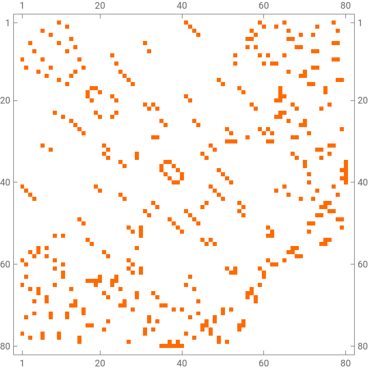
We can now proceed to do graph operations on the skeletal graph, like visualizing the adjacency matrix:
In[]:=
MatrixPlot[AdjacencyMatrix[b80g]]
Out[]=