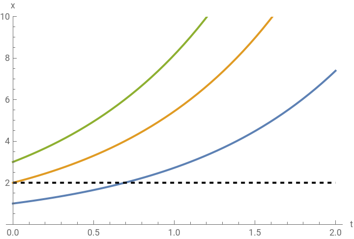
In this study, we addressed a linear first-order hyperbolic partial differential equation (PDE) with an initial value condition. This investigation not only provided insights into the behavior of solutions to linear first-order hyperbolic PDEs but also demonstrated the efficacy of the method of characteristics in solving such equations. The constant solution indicates that the initial condition propagates along the characteristic curves without change, a typical behavior in hyperbolic PDEs representing wave propagation.
The given problem is an initial value problem for .
t>0,x>1
u
t
1
x
u
x
Find the solution and plot the characteristic curves (e . g ., for ).
ξ1,2,3
The given initial value problem is a linear first - order hyperbolic partial differential equation . The method of characteristics is a technique for finding solutions to such equations . Let' s apply it step by step .
1
. Formulation of the Characteristic Equation : The given equation can be written as +0 . This means that the derivatives of with respect to time and space are connected via the relation .
u
t
1
x
u
x
u
t
x
dt
1
dx
1
x
2
. Solving the Characteristic Equation : Solving the above relation, we get the characteristic curves . This can be done through integration : The integration yields : where is a constant of integration that can depend on the initial condition .
dt
dx
x
ln|x|t+C
C
3
. Applying the Initial Condition : The initial condition is . This means that for , for every ) . Substituting this into the characteristic equation, we get :
This means that the constant () is just the logarithm of the initial value of (), i . e ., , where ( ) is the initial value of () .
u(x,0)2
t0
u2
(x>1
ln|x|C
This means that the constant (
C
x
Cln|ξ|
ξ
x
4
. Finding the General Solution : The general solution of the equation is then :
where is an arbitrary function determined by the initial condition . From the initial condition , we get :
This means that is simply the constant function 2.
u(x,t)f(ln|x|-t)
where
f
u(x,0)2
f(ln|x|)2
This means that
f
5
. Final Solution : Thus, the final solution of the equation is : \[\]
The characteristic curves are the lines in the space along which the solution is constant . From the characteristic equation, we have : \[ \]
or
where is the initial value of (e . g ., 1, 2, 3) .
u(x,t)2
The characteristic curves are the lines in the
(x,t)
ln|x|t+ln|ξ|
or
xξ
t
e
where
ξ
x
In[]:=
DSolve[{D[u[x,t],t]+(1/x)D[u[x,t],x]==0,u[x,0]==2},u[x,t],{x,t}]
Out[]=
{{u[x,t]2}}
In[]:=
Show[Plot[{Exp[t],2*Exp[t],3*Exp[t]},{t,0,2},PlotRange->{All,{0,10}},AxesLabel->{"t","x"},PlotLegends->{"x = e^t","x = 2e^t","x = 3e^t"}],Plot[2,{t,0,2},PlotStyle->{Black,Dashed}]]
Out[]=