“Some Mathematical functions are evaluated using power series or rational approximations and whose coefficients are found by some mathematical procedure.
In this project, given known values of mathematical functions, find ANNs that efficiently reproduce the values of the functions and compare their performance with Builtin-Methods and see how the Neural Nets perform on that data.”
In this project, given known values of mathematical functions, find ANNs that efficiently reproduce the values of the functions and compare their performance with Builtin-Methods and see how the Neural Nets perform on that data.”
BesselJ/First Build
BesselJ/First Build
Introduction/Starting Code
Introduction/Starting Code
The first function we decided to try ANNs and approximate was BesseJ, based on SW suggestions, and it would be a good starting point.The function looks like this.

◼
I cannot train it on the whole x Domain, So based on some manual plotting of functions and considering limitations of my four-core CPU. Training domain of 10X10 domain was chosen. If we have the model that works, it most certainly can be extended to a more extensive domain given time/computational resources.During this process, the step size in [x,y] as taken 0.05 for x and 0.01 for y. This decision was made by plotting the graphs. It was small enough so that the training points were close enough for the model to learn and not too close, making our dataset huge and, consequently, longer training times. The reader is encouraged to try different step sizes as he/she likes and see the effects, both on model and training time.
◼
The code to generate data is
data= Table[{x,y} ->N[ BesselJ[x,y]], {x, 0, 10, 0.05},{y,0,10,0.01}]//Flatten;val= RandomChoicedata,Round;data= Complement[data,val]data//Lengthval//Length
Length[data]
10
◼
This will remain, more or less the same throughout the whole process, just with a different step size.
◼
Flatten was used because a Table in multidimensional input generates a nested list, and NetTrain will not interpret those correctly. In case the input is 1-D, Flatten is not required.
◼
After many manual Testing/Tuning, We got some ideas about what things should work and what will not work(I will point the significant observations as we go on).
◼
I have created a bestNetworkFinder. At the moment; It is hard coded to take parameters defined and return a list of NetTrain objects. The function is feasible to use when the user has a limited number of model parameters/net structures, as it saves the user much manual changing of parameters and returns a list of NetTrain objects(For my readers not familiar with WL, these do contain the Trained network and many other model metrics)
◼
Notes to readers
◼
I have added the result of the bestNetworkFinder once; it is too long and entirely unnecessary to show it multiple times. Please let me know if you want the full details. I will be happy to share these with you. Or if you tried something of your own and want to discuss it :).
◼
Some of the points that I noticed but cannot fit in the flow of the document. I have added those in the last section
Results
Results
After the BestNetworkFinder finishes, it is time to get the fruits of your CPU/GPU’s labor, and we get all of the models. Note: The model giving the lowest Mean square error or Mean L2-Norm is not always the best choice (as highlighted later). Back to BesselJ, the least MSE, as in most cases, did work the best.
With model parameters and training code:
With model parameters and training code:
schedule[b_,bmax_]:=(1-b/bmax);bJP=NetTrain[NetChain[{400,Ramp,400,Tanh,400,1}],data,All,MaxTrainingRounds->400,TargetDevice"GPU",BatchSize64,LearningRate,Method{"SignSGD","LearningRateSchedule"schedule},ValidationSetval]
-4
10
◼
Which Gave the resultant Model as
NetTrainResultsObject

◼
As you can see the MSE values were pretty low, but the mean values doesn’t always shows the best results. So lets see the error graph

◼
I would not bore you with same code again and again, so I have mentioned how to get the graph in Spherical Harmonics of cause BesselJ takes an hour to train, and SphericalHarmoincs just takes 5, so easier to evaluate again.
0
Y
2
Angular Part of wavefunction of hydrogen atom:
Angular Part of wavefunction of hydrogen atom:
The solution of the wavefunction of the electron in a single electron hydrogen atom is given by:
phi[n_,l_,m_]=***LaguerreLn-l-1,2l+1,SphericalHarmonicY[l,m,θ,ϕ]a=52.9*
3
2
n a
(n-l-1)!
2n*()
3
((n+l)!)
-r
n a
l
2r
n a
2r
n a
-12
10
Where n,l, and m are the quantum numbers.
a is Bohr radius.
r,θ,ϕ are the spherical coordinates
Approximating the whole function would have been difficult, so as any derivation of this equation is done, we will do both parts separately.
a is Bohr radius.
r,θ,ϕ are the spherical coordinates
Approximating the whole function would have been difficult, so as any derivation of this equation is done, we will do both parts separately.
Introduction / General Remarks
Introduction / General Remarks
◼
The basic process for finding the NN approximations for the [n,l,θ,ϕ] is the same as BesselJ, albeit making little changes in the model size.
◼
The model was trained on ,it gives us the probability density, helps us in visualization things, and keeps our output Real.
The code used is:
2
Norm[SphericalHarmonicY[l,m,x,y]]
The code used is:
data= Table[{x,y} ->//N, {x, 0, 2π, 0.001π},{y,0,2π,0.2π}]//Flatten;val= RandomChoicedata,Round;data= Complement[data,val];data//Lengthval//Length
2
Norm[SphericalHarmonicY[l,m,x,y]]
Length[data]
10
◼
The domain was not a problem in this case since θ and ϕ take values [0,2π]and will be periodic after . If we have the model that works, it most certainly coded to reduce the arguments to [0,2π].During this process, the step size in [l,m,x,y] taken 0.001π for x and 0.2π for y. This decision was made by plotting the graphs and since the value of the function does not change with Norm^2 of the function. It was small enough so that the training points were close enough for the model to learn. The reader is encouraged to try different step sizes as he/she likes and see the effects, both on model and training time. One interesting point to note is that, even if the training data was constant with respect to y, there were still slight variations in the trained models if we change y.
◼
It is observed that the basic Net structure of {LinearLayer,Ramp(Also known as Relu),LinearLayer,Tanh,Output} was enough to produce good results. We just needed to change the size/no of perceptrons of the layers and tinker with learning rates/Optimizers. I hypothesize that since the functions(including) are smooth curves, the same kind of model did work for all of these functions. We just needed to increase the size of the layers as function complexity increased. Models were also made by adding more layers; some work for better, some worse, some start overfitting, or have marginal changes. More exploration is required.
Results/Graphs :
Results/Graphs :
Keeping the last point in mind, I will not not make the post abruptly long by adding each of the network that came out of bestNetworkFinder, I’ll instead Tabulate the results and point out the interesting observations/graphs with code to generate them.
Out[]=
l,m | Function | Training Domain | MSE(Training set) | MSE(Validation Set) |
1,0 | Norm[SphericalHarmonicY[1,0,x,y] 2 ] | 2π x 2π on | 1.62 x -8 10 | 1.41 x -8 10 |
1,1 | Norm[SphericalHarmonicY[1,1,x,y] 2 ] | 2π x 2π on | 9.52 x -10 10 | 9.73 x -10 10 |
1,-1 | Norm[SphericalHarmonicY[1,-1,x,y] 2 ] | 2π x 2π on | 3.07 x -9 10 | 2.91 x -9 10 |
2,2 | Norm[SphericalHarmonicY[2,2,x,y] 2 ] | 2π x 2π on | 3.91 x -9 10 | 3.98 x -9 10 |
2,-2 | Norm[SphericalHarmonicY[2,-2,x,y] 2 ] | 2π x 2π on | 3.98 x -9 10 | 3.65 x -9 10 |
2,0 | Norm[SphericalHarmonicY[2,0,x,y] 2 ] | 2π x 2π on | 2.99 x -7 10 | 2.54 x -7 10 |
2,1 | Norm[SphericalHarmonicY[2,1,x,y] 2 ] | 2π x 2π on | 7.32 x -8 10 | 8.43 x -8 10 |
2,-1 | Norm[SphericalHarmonicY[2,-1,x,y] 2 ] | 2π x 2π on | 8.59 x -8 10 | 9.03 x -8 10 |
◼
You might notice some run to run variance as the validation data is randomly selected from training data and random initial weights and biases. As seen in the last two columns, the function effectively is the same.
◼
Among the grid search between given Optimizers in WL and learning rates, the Best ones were “RMSProp” and “SignSGD” with learning rate in range ] with schedule as given above
[,
-4
10
-6
10
Error Graphs/Observations
Error Graphs/Observations
◼
0
Y
1
◼
The net was prepared as
◼
hen the list and graph of error vs. x are produced since y is not affecting the list much. It is a 1D plot to show the characteristics better. I will show the 3D plot in the 3rd item.
◼
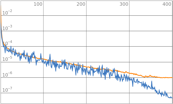
This is a case which shows Blindly trusting Mean Square Error is not a good strategy, as in this case the errors were concentrated in some region and were very low for others
◼
The code to get the model is
◼
Which gave the model
◼
This is not even close what is intuitive from MSE value, but it is Mean values and in some cases might not show the full picture
Radial Part
Radial Part
◼
The basic process for finding the NN approximations for the Radial Part is same as the previous two.
Results/Graphs
Results/Graphs
◼
As mentioned before, I’ll Tabulate the results and point out the interesting observations/graphs with code to generate them.
◼
Among the grid search between given Optimizers in WL and learning rates, the Best ones were “Adam,” “RMSProp,” and “SignSGD” with learning rate in the range [10^-3,10^-5] with schedule as given above.
◼
These did require a few layers of {Ramp,LinearLayer} for more complicated curves of n=3
◼
Furthermore, the Radial part did require more epochs, up to 625, depending upon the size of the model/complexity of the function.
◼
I will add some of the error curves, and the rest follow a similar trend. All are prepared using the same code, as mentioned in the previous section.
◼
1s
◼
2s
◼
The magnitude of error increased as the function approached zero, I guess either training time/model was little bit short
◼
2p
◼
3d
FuncNets for complex functions:
FuncNets for complex functions:
I could not finish an extensive analysis as I would have liked to, given the two week time limits
The function I chose to train upon is, as it gave both
The function I chose to train upon is, as it gave both
First I tried to train on a 10 x 10 domain for {x+ y}, but small increment in x and y would make huge changes in the output of the function. So we needed a huge dataset, well that could not be done due to computational resource limitations.
Then i tried to cheat around it and try to train the model on a unit circle in the Complex Plane, by using the following code
Then i tried to cheat around it and try to train the model on a unit circle in the Complex Plane, by using the following code
This would map x to the circle in Complex Plane, but I have tried most structures of NNs I could think of(its not exhaustive , of course ,I had time limitations, but tried many things). I could not reliably produce a good approximation.
So, in our next attempt I made the input vector as 2-D and generated the data as:
Then I did train a few models manually this time, cause each took about an hour, because our training data points needed to be close to a million for even 1x1 grid.
It gave the following model as result, and the predicted values look very close to actual values, but further detailed analysis is incomplete, when I do pursue it further.I will make sure to update the post.
Concluding remarks
Concluding remarks
Thank You so much for reading. If you have any ideas/suggestions/comments. Or you would like to discuss more, feel free to let me know. I will be more than happy to do that.
Future plans/Ideas
Future plans/Ideas
◼
A more detailed analysis of complex functions based upon previous experience.
◼
Try our more different kinds of neural nets.
◼
Observe how the model behaves as a function of model complexity/Training Time.
◼
Explore it on different functions, mainly polynomials, and how far we can stretch these.
Keywords
Keywords
◼
FuncNets
◼
ANN
◼
Functional Approximation
◼
Rahul Sharma
◼
Hydrogen Atom
◼
BesselJ
Acknowledgment
Acknowledgment
A huge acknowledgment and Thanks to my mentor Tuseeta Banerjee. Without her help, the project would not be possible.
Stephen Wolfram for his input.
Jessie, Silvia, and all the TA’s for answering my stupid questions, you guys are the best.
All the teachers for their knowledge they gave us.
Mads for being an awesome director.
And a special thanks to all my fellow participants who made my time in WSS memorable. See you around.
Stephen Wolfram for his input.
Jessie, Silvia, and all the TA’s for answering my stupid questions, you guys are the best.
All the teachers for their knowledge they gave us.
Mads for being an awesome director.
And a special thanks to all my fellow participants who made my time in WSS memorable. See you around.