Quadratically increasing CO2 emission will increase CO2 concentration cubically and also the Earth’s temperature
Quadratically increasing CO2 emission will increase CO2 concentration cubically and also the Earth’s temperature
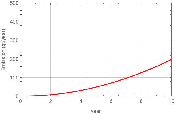
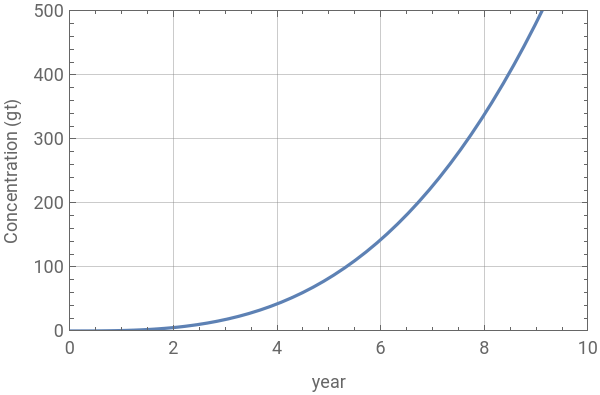
This is to demonstrate that as CO2 emissions (inflow, gigatons/year) increase quadratically (2nd order), the CO2 concentration (or atmospheric CO2 in gigatons, gt) will increase cubically (3rd order). Therefore, it can be logically concluded that Earth’s temperature will increase non-linearly (much faster) as there is a relationship between atmospheric CO2 and temperature. I used the relationship between speed and distance as an analogy.
◼
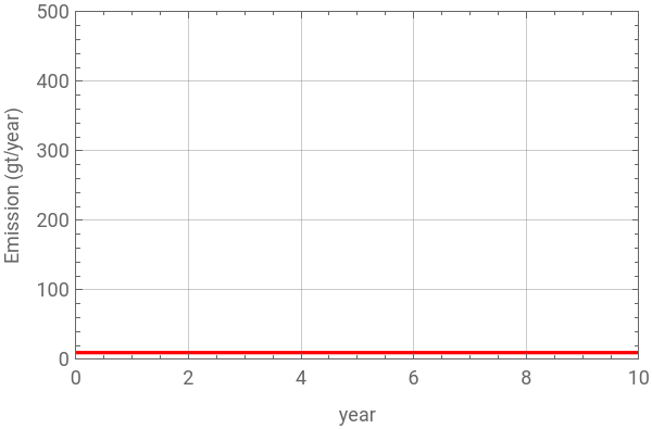
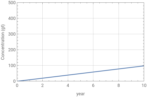
If CO2 emission is constant, then CO2 concentration will increase linearly over time.
◼
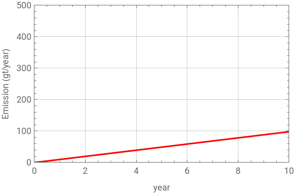
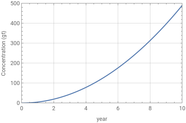
If CO2 emission increase linearly, then CO2 concentration will increase quadratically over time.
◼
If CO2 emission increase quadratically, then CO2 concentration will increase cubically (3rd order).
Analogy : {speed (meter/second) vs. distance (meter)} and {CO2 emission (gt/year) vs. CO2 concentration (gt)}
Analogy : {speed (meter/second) vs. distance (meter)} and {CO2 emission (gt/year) vs. CO2 concentration (gt)}
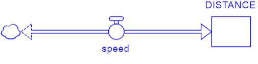

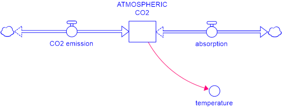
Speed and distance
Speed and distance
◼
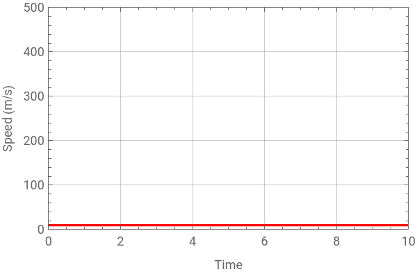
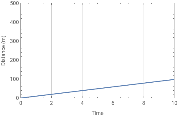
Case 1. Speed is constant
In[]:=
sol=DSolve[{x'[t]9.8,x[0]0},x,{t,0,10}]
Out[]=
{{xFunction[{t},0.+9.8t]}}
{Plot[{x'[t]/.sol},{t,0,10},FrameTrue,FrameLabel{"Time","Speed (m/s)"},PlotLegendsPlaced[{"Speed (m/s)"},Above],PlotRange{{0,10},{0,500}},GridLinesAutomatic,ImageSize300,PlotStyleRed],Plot[{x[t]/.sol},{t,0,10},FrameTrue,FrameLabel{"Time","Distance (m)"},PlotLegendsPlaced[{"Distance (m)"},Above],PlotRange{{0,10},{0,500}},GridLinesAutomatic,ImageSize300]}//Row
Out[]=


◼
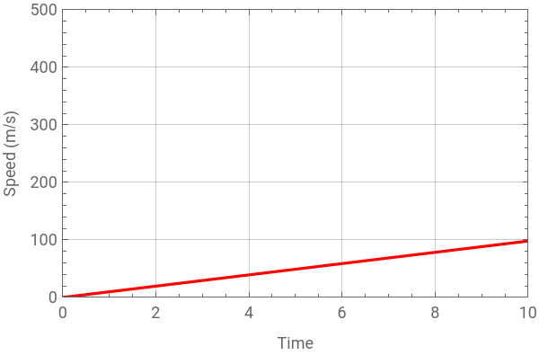
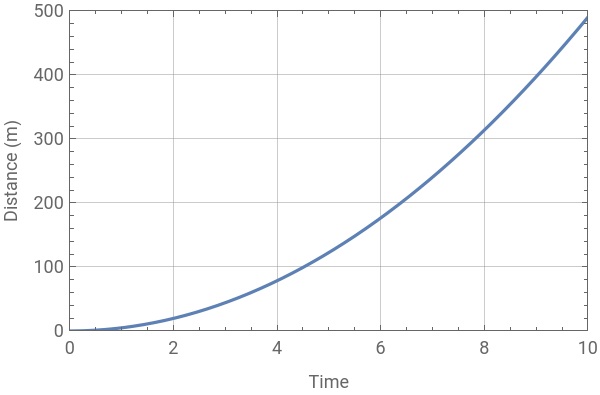
Case 2. Speed increases linearly
In[]:=
sol2=DSolve[{x'[t]9.8*t,x[0]0},x,{t,0,10}]
Out[]=
{{xFunction[{t},4.9]}}
2
t
{Plot[{x'[t]/.sol2},{t,0,10},FrameTrue,FrameLabel{"Time","Speed (m/s)"},PlotLegendsPlaced[{"Speed (m/s)"},Above],PlotRange{{0,10},{0,500}},GridLinesAutomatic,ImageSize300,PlotStyleRed],Plot[{x[t]/.sol2},{t,0,10},FrameTrue,FrameLabel{"Time","Distance (m)"},PlotLegendsPlaced[{"Distance (m)"},Above],PlotRange{{0,10},{0,500}},GridLinesAutomatic,ImageSize300]}//Row
Out[]=
◼
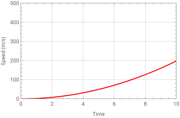
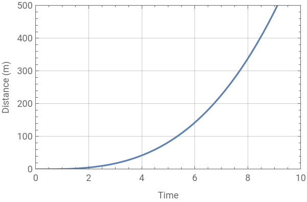
Case 3. Speed increases quadratically
In[]:=
sol3=DSolve[{x'[t]1.98*t^2,x[0]0},x,{t,0,10}]
Out[]=
{{xFunction[{t},0.66]}}
3
t
In[]:=
{Plot[{x'[t]/.sol3},{t,0,10},FrameTrue,FrameLabel{"Time","Speed (m/s)"},PlotLegendsPlaced[{"Speed (m/s)"},Above],PlotRange{{0,10},{0,500}},GridLinesAutomatic,ImageSize300,PlotStyleRed],Plot[{x[t]/.sol3},{t,0,10},FrameTrue,FrameLabel{"Time","Distance (m)"},PlotLegendsPlaced[{"Distance (m)"},Above],PlotRange{{0,10},{0,500}},GridLinesAutomatic,ImageSize300]}//Row
Out[]=
CO2 emission and concentration
CO2 emission and concentration
◼
Case 1. CO2 emission (giga tons / year) is constant
In[]:=
solC=DSolve[{concentration'[t]9.8,concentration[0]0},concentration,{t,0,10}]
Out[]=
{{concentrationFunction[{t},0.+9.8t]}}
In[]:=
(*Thevaluesusedforco2emissionandconcentrationareusedasademonstrationanddonotreflecttheactualvalues*){Plot[{concentration'[t]/.solC},{t,0,10},FrameTrue,FrameLabel{"year","Emission (gt/year)"},PlotLegendsPlaced[{"Emission (gt/year)"},Above],PlotRange{{0,10},{0,500}},GridLinesAutomatic,ImageSize300,PlotStyleRed],Plot[{concentration[t]/.solC},{t,0,10},FrameTrue,FrameLabel{"year","Concentration (gt)"},PlotLegendsPlaced[{"Concentration (gt)"},Above],PlotRange{{0,10},{0,500}},GridLinesAutomatic,ImageSize300]}//Row
Out[]=
◼
Case 2. CO2 emission (giga tons / year) increases linearly
In[]:=
sol2C=DSolve[{concentration'[t]9.8*t,concentration[0]0},concentration,{t,0,10}]
Out[]=
{{concentrationFunction[{t},4.9]}}
2
t
In[]:=
{Plot[{concentration'[t]/.sol2C},{t,0,10},FrameTrue,FrameLabel{"year","Emission (gt/year)"},PlotLegendsPlaced[{"Emission (gt/year)"},Above],PlotRange{{0,10},{0,500}},GridLinesAutomatic,ImageSize300,PlotStyleRed],Plot[{concentration[t]/.sol2C},{t,0,10},FrameTrue,FrameLabel{"year","Concentration (gt)"},PlotLegendsPlaced[{"Concentration (gt)"},Above],PlotRange{{0,10},{0,500}},GridLinesAutomatic,ImageSize300]}//Row
Out[]=
◼
Case 3. CO2 emission (giga tons / year) increases quadratically. This reflects current economic development and has implications to Earth temperature
In[]:=
sol3C=DSolve[{concentration'[t]1.98*t^2,concentration[0]0},concentration,{t,0,10}]
Out[]=
{{concentrationFunction[{t},0.66]}}
3
t
{Plot[{concentration'[t]/.sol3C},{t,0,10},FrameTrue,FrameLabel{"year","Emission (gt/year)"},PlotLegendsPlaced[{"Emission (gt/year) increases quadratically"},Above],PlotRange{{0,10},{0,500}},GridLinesAutomatic,ImageSize300,PlotStyleRed],Plot[{concentration[t]/.sol3C},{t,0,10},FrameTrue,FrameLabel{"year","Concentration (gt)"},PlotLegendsPlaced[{"Concentration (gt) increase cubically"},Above],PlotRange{{0,10},{0,500}},GridLinesAutomatic,ImageSize300]}//Row
Out[]=
CITE THIS NOTEBOOK
CITE THIS NOTEBOOK
Current CO2 emission will increase CO2 concentration cubically
by Sangdon Lee
Wolfram Community, STAFF PICKS, May 20 2023
https://community.wolfram.com/groups/-/m/t/2922562
by Sangdon Lee
Wolfram Community, STAFF PICKS, May 20 2023
https://community.wolfram.com/groups/-/m/t/2922562