By approximating 2-Manifolds in with polyhedra and then converting them into graphs weighted by Euclidean length of the edges, we can use graph theoretic methods to study the properties of the underlying mesh. By assuming the existence of a graph version of the Bertrand-Diguet-Puiseux Theorem and finding a graph equivalent of geodesic disks, it is possible to estimate relative curvatures on the surface by taking the new graph curvatures of the points along the approximation. By using the number of new vertices as a metric for the rate of change of the area of the geodesic disk, we can perform a regression, so by L’Hôpitals’s theorem, the resulting metric is approximately negatively proportional to the true Gaussian curvature at the point. This varies from previous measures of discrete curvature that use angles around points.
3
R
Introduction
Introduction
My goal for this project was to create a new way of estimating the curvature of polyhedra. The traditional method uses the angle deficits around vertices. It is possible to define the curvature using a geodesic disk by the Bertrand - Diguet - Puiseux Theorem. A geodesic disk is all points within a certain distance on a surface from a given point. This is important because it is easy to approximate distances on a surface from a graph that approximates by simply taking the shortest graph distance between 2 points. This led me to believe that it was possible to approximate the relative curvature of a 2-Manifold by taking the relative rates of growth of concentric circles around the point in . However it is difficult to exactly calculate the area of geodesic disk around each point, especially if the manifold is artificially contrived. So I the graph approximation. These graphs are constructed from the edges of triangulations of the surfaces. I found that fairly accurate relative curvature measurements are possible. This has possible applications in computer graphics as they often attempt to approximate smooth surfaces with polyhedra. This has applications in computer graphics as computers render 3D shapes using triangulated meshes and it is easy for computers to determine the distance between two points. It could also possibly have impacts in relativity as an alternative to Regge calculus, a method of determining the shape of the spacetime manifold.
The Bertrand-Diguet-Puiseux Theorem states:
The Bertrand-Diguet-Puiseux Theorem states:

By understanding that the top and bottom approach 0, we can see that the limit on the right is indeterminate assuming A(r) approaches 0 so we can use L’Hôpital’s with respect to r to get new equivalent relation .
Theorem 1.1:
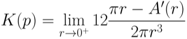
L’Hôpital’s rule may be applied again to get:
Theorem 1.2:
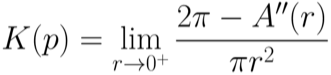
This shows that the second derivative of A(r) can be used as an approximation for curvature when expanding the circle rather than shrinking it. This however only holds for smooth surfaces. The main intuition behind my project is that if a geodesic disk is all points within a graph distance r from p, then A’(r) would be the number of new dots at each increment of r, N(r). Finally, A’’(r) would be the rate of change of this number of new dots or N’(r) We can estimate N’ by performing a linear regression on values of N for increasing r. This is the key insight, the slope of that linear regression can be used to approximate the curvature, and the backbone of my project.
Understanding Curvature
Understanding Curvature
What Is Curvature
What Is Curvature
Gaussian Curvature
Gaussian Curvature
Gaussian curvature (K) is a measure of how much a surface bends. The Gaussian curvature at a point (K) is the product of the curvature of the 2 geodesic lines at the point with the most and least curvature, called the principle curvatures. Intuitively this means if they both bend in the same direction then K will be positive, like every point on a sphere; If they bend in opposite directions K will be negative, like in a saddle; and if one of the lines is straight, like in a cylinder then both the curvature will be 0.
What does it mean for a polyhedra to be curved?
What does it mean for a polyhedra to be curved?
The concept of curvature is much more difficult to define on polyhedra because every principle curvature has curvature 0. as they are straight lines.
A traditional method to approach a good approximation is to take the deficit from 360 degrees of a vertex on the polyhedra. In fact for certain triangulation conditions, the metric converges to the true gaussian curvature that a polyhedra is approximates. However the method I used was based on approximating the area of geodesic disks on polyhedra, something that can be defined on a polyhedra, by the number of vertices within a certain graph distance of a vertex.
A traditional method to approach a good approximation is to take the deficit from 360 degrees of a vertex on the polyhedra. In fact for certain triangulation conditions, the metric converges to the true gaussian curvature that a polyhedra is approximates. However the method I used was based on approximating the area of geodesic disks on polyhedra, something that can be defined on a polyhedra, by the number of vertices within a certain graph distance of a vertex.
Method
Method
Overview
Overview
The process starts with converting some smooth shape or region into a triangulated polyhedra. I then convert the polyhedra to a graph with the edge weights proportional to their euclidean lengths. Then for each point in the graph the code iterates out counting how many new points are included each time you increase the radius, it then performs a linear regression and use the slope as a measure of relative curvature. We can do this because of theorem 1.2. It is essentially measuring the rate at which a geodesic disk grows in area around a point. If the graph has negative curvature then the returned metric will be higher, if the graph has positive curvature, then the metric will be lower. If you iterates the check over each vertices you can get the approximate relative curvature across the surface.
Code Overview
Code Overview
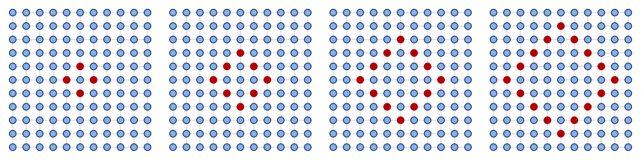
The boundary function returns all nodes in a graph between graph distance r-1 and r away from a given node.
Clear[boundary]boundary[g_,c_,r_]:=Join[DeleteElements[AdjacencyList[g,c,r],AdjacencyList[g,c,r-1]],{c}]
Highlight the vertices returned by boundary for various radii
Out[]=
graphReg=Remeshr0,;
The function converts the polyhedra into a graph by using the vertices of the polyhedra as the nodes of the graph.
meshFrame=meshReg//MeshConnectivityGraph;
Finally the function weighs each edge by its euclidean distance, further increasing the accuracy of distance measurements along the graph.
weights=meshReg//MeshPrimitives[#,1]&//Map[First/*Differences/*Norm];MeshConnectivityGraph[meshFrame,EdgeWeight->weights,VertexSize->Large]
The final code then returns this weighted graph which can be used for the curvature computation.
ClearAll[meshFrame,meshReg,weights,meshGraph]meshGraph[r_]:= Module[{r0=r, meshReg, meshFrame,weights},meshReg=Remesh[r0,Method->{"Adaptive",{"MaxEdgeLength"->.1`,"MinEdgeLength"->0.05`}}]; weights=meshReg//MeshPrimitives[#,1]&//Map[First/*Differences/*Norm];Graph[MeshConnectivityGraph[meshReg],EdgeWeight->weights,VertexSize->Large]]
The curvature function is the back-bone of the project. It iterates over the points near a vertex in the graph and plots the growth of the
boundary. I then takes a regression on the data and returns the slope. This, in a perfectly smooth manifold, would be negatively proportional to the curvature.
boundary. I then takes a regression on the data and returns the slope. This, in a perfectly smooth manifold, would be negatively proportional to the curvature.
Clear[curvature]curvature[g_, n_] := Module[{n0 = n, t, lm, g0 = g}, t = Table[{i, Length[Boundary[g,n,i]]}, {i, 1, sampleLength}]; lm = LinearModelFit[t, x, x]; lm["BestFitParameters"][[2]]];
Finally, the function that I use to visualize my curvature metric scales the maximum and minimum curvature between 0 and 1 on a graph and maps each vertex on the graph to the color associated with its curvature.
It calculates the curvature of each vertex on the graph and saves it to a variable.
It calculates the curvature of each vertex on the graph and saves it to a variable.
curvs=ParallelTable[curvature[g,v],{v,VertexList[g]}];
ClearAll[ curvs, curvMap, maxDist];highlightCurvs[meshGraph_]:=Module[{g=meshGraph, curvs, maxDist, minDist,curvMap},curvs = ParallelTable[curvature[g, v], {v, VertexList[g]}];maxDist = Max[Flatten[curvs]];minDist = Min[Flatten[curvs]];curvMap = AssociationThread[VertexList[g] -> curvs];HighlightGraph[g, ParallelTable[ With[{scaledDist = Clip[1-Rescale[curvMap[v], {minDist, maxDist}], {-1, 1}]}, Style[v, ColorData["SunsetColors"][scaledDist]] ], {v, VertexList[g]} ], VertexSize->5]]
Exploring Meshes
Exploring Meshes
A torus is an excellent shape to test the function on as it has very clear regions of high and low curvature. The principles curvatures are around the big ring, and around the tube of the torus. Since theses bend away from each other on the inside of the torus,
Initialize the torus mesh
Initialize the torus mesh
In[]:=
torusMesh=DiscretizeRegion[Torus[{0,0,0},{1,2}]]
Out[]=
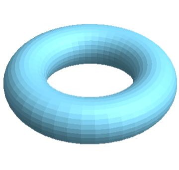
We triangulate the mesh and then convert the output to a weighted graph in order to make measurements of distance along the graph as accurate as possible.
In[]:=
tGraph=meshGraph[torusMesh]
Out[]=

Color the graph based on the calculated curvature metric at
In[]:=
sampleLength=20;highlightCurvs[tGraph]
Out[]=

One can see that the model accurately determines the relative curvature on the torus. This is interesting because the only information it reattained from the original torus was the distance between vertices in the form of edge weights and the edges themselves as the connections between nodes. While our embedding is specifically still in the shape of a torus it doesn’t necessarily have to. be. This is where the power of this model comes from. It is able to determine a physical property of what it is approximating while retaining very little information.
Another example with clearly defined relative curvatures is an ellipsoid. The points at the tips should have the highest curvature and the points on the flat side should have the lowest.
Initialize the ellipsoid
Convert mesh to triangulated weighted graph in order to once again make measurements of distance along the graph as accurate as possible
Color the graph vertices based on the curvature of the ellipsoid
Initialize mesh based on inequality
Convert mesh to graph
Color the graph vertices based on the curvature of the shape
One can see the algorithm does a good job of getting relative curvatures. However, it sometimes fails to be precise as one can see along the flat sides of the ellipsoid, where there is variation in colors where there shouldn’t be.
Conclusion
Conclusion
Implications
Implications
As stated in the introduction, there have been other methods used in the past for determining the curvature of smooth meshes using polyhedra approximations. However they usually rely on knowing the angles of triangles around each point. This method allows us to reconstruct the curvature using even less information about the underlying surface. This could have implications in computer graphics and other areas that rely on discrete geometry.
Limitations
Limitations
While my code could effectively get the relative curvatures across the graph, it is not very efficient. It requires calculating the number of neighbors at each point at different radii across every point in a graph. It also relies on the definition of the graph in order to be accurate to the surface it is approximating. This leads to certain areas not being very precisely measured leading to variations over regions that should have the same curvature, as mentioned above on the ellipsoid. However, in order for the the code to capture these nuances, the graph would need to be have a large number of vertices, and it could be very computationally expensive. The approximations are also reliant on the sample length as too short and the metric doesn’t capture any curvature, but too long and it captures the curvature of points around it.
Future Direction
Future Direction
While the work I have done have interesting applications, there are also many ways I would like to expand in the future. The first way is in exploring higher dimensional manifolds. By using graph approximations of 3-manifolds embedded in 4D space, It could be possible to get an approximation of the curvature of the underlying manifold. This could be used as an alternative to Regge calculus in determining the relative curve of space time across a region, possibly using light speed to accurately calculate accurate geodesic distances. I would also like to provide a conjecture:
Conjecture 1:
The limit of the BDP-theorem evaluated on a polyhedra approximation will converge to real gaussian curvature of a smooth manifold under sufficient conditions, as the polyhedra becomes a better approximation of the underlying smooth manifold.
Conjecture 1:
The limit of the BDP-theorem evaluated on a polyhedra approximation will converge to real gaussian curvature of a smooth manifold under sufficient conditions, as the polyhedra becomes a better approximation of the underlying smooth manifold.
I would like to prove this conjecture however it is outside the scope of what I could accomplish in 2 weeks.
Acknowledgements
Acknowledgements
I would like to thank the Wolfram Summer Research Program, Stephen Wolfram, Dugan Hammock, the directors, my T.A. Eric and the rest of the TAs of the program. Additional thanks to Stephen Wolfram for suggesting this project.
References
References
Contributors to Wikimedia projects. (2003, July 31). Gaussian curvature. Wikipedia.Org; Wikimedia Foundation, Inc. https://en.wikipedia.org/wiki/Gaussian_curvature
Contributors to Wikimedia projects. (2008, August 8). Bertrand-Diguet-Puiseaux Theorem. Wikipedia.Org; Wikimedia Foundation, Inc. https://en.wikipedia.org/wiki/Bertrand%E2%80%93Diguet%E2%80%93Puiseux_theorem
GATZKE, T. D., & GRIMM, C. M. (2006). ESTIMATING CURVATURE ON TRIANGULAR MESHES. International Journal of Shape Modeling, 12(01), 1–28. https://doi.org/10.1142/s0218654306000810Makovník, M., & Pavel, C. (2023).
Curvature estimation for meshes via algebraic quadric fitting. arXiv.Org. https://arxiv.org/abs/2304.08909
Wikipedia Contributors. (2026, February 21). Regge calculus. Wikipedia; Wikimedia Foundation. https://en.wikipedia.org/wiki/regge_calculus
CITE THIS NOTEBOOK
CITE THIS NOTEBOOK
A novel approach for recovering curvature of smooth surfaces in 3D from graph approximation
by Winston Garcia
Wolfram Community, STAFF PICKS, July 9, 2026
https://community.wolfram.com/groups/-/m/t/3752948
by Winston Garcia
Wolfram Community, STAFF PICKS, July 9, 2026
https://community.wolfram.com/groups/-/m/t/3752948