Establishing maximal entanglement speed via branchial lightcones
By: William Munizzi
Work conducted as part of the Wolfram Summer School 2022
By: William Munizzi
Work conducted as part of the Wolfram Summer School 2022
Abstract
Abstract
The rate of entanglement provides a speed limit for information propagation through branchial space. Just as event horizons demonstrate causally disconnected regions of spacetime, so too can branchial divergence indicate regions where entanglement forbidden. An observer traveling along some geodesic confined to the disconnected region of branchial space would then need to exceed some maximal entanglement speed to escape the region. We consider an initially pure system of qubits, under evolution of some quantum circuit, and investigate the maximal entanglement rate and its implications for the physical observer.
Function Definitions (Run this Section)
Function Definitions (Run this Section)
Introduction and Examples of Functionality
Introduction and Examples of Functionality
In this notebook we model the evolution of systems of qubits, and their associated properties, under different quantum circuits. A quantum circuit consists of an initial quantum state of n qubits, that is evolved in time by the subsequent application of chosen quantum gates. The physical state may be represented as a vector of length , with each component the particular coefficient multiplying one of the computational basis kets spanning the ambient Hilbert space. At three qubits, these coefficients would multiply the basis {{000}, {001}, {010}, {011}, {100}, {101}, {110}, {111}}, in that progressive order. As an example, the 3-qubit GHZ state may be written ,{0}, {0}, {0}, {0}, {0}, {0}, , an equal-probability superposition of the “all-up” and “all-down” states. In this project, we further adopt a bit-address normalization scheme that sets the first non-zero component to 1, e.g. the same 3-qubit GHZ will be written {{1},{0}, {0}, {0}, {0}, {0}, {0}, {1}}. The bit-address representing the product state of n single qubits can be built using the Kronecker product,
n
2
1
2
1
2
KroneckerProduct[{{1},{0}},{{1},{0}},{{0},{1}}]KroneckerProduct[{{1},{0}},{{0},{1}},{{1},{0}}]KroneckerProduct[{{0},{1}},{{1},{0}},{{1},{0}}]
Out[]=
{{0},{1},{0},{0},{0},{0},{0},{0}}
Out[]=
{{0},{0},{1},{0},{0},{0},{0},{0}}
Out[]=
{{0},{0},{0},{0},{1},{0},{0},{0}}
Accordingly, quantum gates may be represented as matrices that transform one state vector to another. Single-qubit gates are those whose action affects only one qubit in a multi-qubit system, whereas multi-qubit gates can affect several. The full state vector of n-qubits is evolved by a )matrixcomposed of tensor products of single/multi-qubit action, with the identity element acting on all untargeted qubits. Quantum gates in this notebook are initiated by calling the function bearing their name, along with arguments for overall dimension of the system and the qubit to be acted upon.
As an example, to act with a Hadamard gate on the first qubit of the 3-qubit GHZ state, one would call
(x
n
2
n
2
As an example, to act with a Hadamard gate on the first qubit of the 3-qubit GHZ state, one would call
HadamardGate[3,1].{{1},{0},{0},{0},{0},{0},{0},{1}}
Out[]=
,,{0},{0},{0},{0},,-
1
2
1
2
1
2
1
2
Converting this ket to our chosen normalization scheme can be done with the RepresentationNorm[] function, inputting the unnormalized vector as argument,
RepresentationNorm,,{0},{0},{0},{0},,-
1
2
1
2
1
2
1
2
Out[]=
{{1},{1},{0},{0},{0},{0},{1},{-1}}
Similarly, acting on the same state with a CNOT gate that uses the first qubit as control and the third qubit as a target would yield,
CNOTGate[3,{1,3}].{{1},{0},{0},{0},{0},{0},{0},{1}}
Out[]=
{{1},{0},{0},{1},{0},{0},{0},{0}}
Simulation of a designed circuit then proceeds with subsequent gate action on an initial state. As an example, consider the circuit that builds that 3-qubit GHZ state from the 3-qubit vacuum (the 3-fold tensor product of the lowest energy “down” state). The circuit consists of a Hadamard gate applied to the first qubit, followed by two CNOT gates affecting qubits 1 and 2, and 2 and 3 respectively,
CNOTGate[3,{2,3}].CNOTGate[3,{1,2}].HadamardGate[3,1].{{1},{0},{0},{0},{0},{0},{0},{0}}
Out[]=
,{0},{0},{0},{0},{0},{0},
1
2
1
2
For purposes of rewriting rules, it may be convenient to represent a quantum state as a bit-string. Converting a quantum state from its vector notation to a string notation can be accomplished with the QuantumToString[] function,
QuantumToString[{{1},{0},{0},{1},{0},{0},{0},{0}}]QuantumToString,{0},{0},{0},{0},{0},{0},QuantumToString[{{0},{1},{0},{0},{0},{0},{0},{0}}]
1
2
1
2
Out[]=
{{1}, {0}, {0}, {1}, {0}, {0}, {0}, {0}}
Out[]=
{{1}, {0}, {0}, {0}, {0}, {0}, {0}, {1}}
Out[]=
{{0}, {1}, {0}, {0}, {0}, {0}, {0}, {0}}
Quantum states in a string representation can be transformed directly by quantum gates with the StringTransform[] function. The user need only input the string representing the state, followed by the desired gate to evolve the system,
StringTransform[QuantumToString[{{1},{0},{0},{1},{0},{0},{0},{0}}],HadamardGate[3,1]]StringTransform[QuantumToString[{{1},{0},{I},{0},{1},{0},{0},{I}}],TGate[3,2]]StringTransform[QuantumToString[{{1},{0},{0},{0},{0},{0},{0},{I}}],PhaseGate[3,1].HadamardGate[3,1]]StringTransform[QuantumToString[{{1},{1},{1},{1},{1},{1},{1},{1}}],CNOTGate[3,{1,2}].HadamardGate[3,1].TGate[3,2]]
Out[]=
{{1}, {1}, {1}, {-1}, {0}, {0}, {0}, {0}}
Out[]=
{{1}, {0}, {I*E^((I/4)*Pi)}, {0}, {1}, {0}, {0}, {I*E^((I/4)*Pi)}}
Out[]=
{{1}, {I}, {0}, {0}, {0}, {0}, {I}, {1}}
Out[]=
{{1}, {0}, {E^((I/4)*Pi)}, {0}, {1}, {0}, {E^((I/4)*Pi)}, {0}}
The mathematical group generated by the Hadamard, Phase, and CNOT operations is known as the Clifford group. This group has several special properties that render it an interesting point of study. For one, quantum circuits built of Clifford group operations can be efficiently simulated on a classical computer. Additionally, simple models of discrete error-correction employ Clifford operations for error syndrome-diagnosis and recovery. The set of Clifford generators for n-qubits can be assembled, in their matrix form, using the CliffordGenerators[Dimension] function, for example,
MatrixForm/@CliffordGenerators[2]
Out[]=
,
,
,
,
,
1 2 | 1 2 | 0 | 0 |
1 2 | - 1 2 | 0 | 0 |
0 | 0 | 1 2 | 1 2 |
0 | 0 | 1 2 | - 1 2 |
1 2 | 0 | 1 2 | 0 |
0 | 1 2 | 0 | 1 2 |
1 2 | 0 | - 1 2 | 0 |
0 | 1 2 | 0 | - 1 2 |
1 | 0 | 0 | 0 |
0 | | 0 | 0 |
0 | 0 | 1 | 0 |
0 | 0 | 0 | |
1 | 0 | 0 | 0 |
0 | 1 | 0 | 0 |
0 | 0 | | 0 |
0 | 0 | 0 | |
1 | 0 | 0 | 0 |
0 | 0 | 0 | 1 |
0 | 0 | 1 | 0 |
0 | 1 | 0 | 0 |
1 | 0 | 0 | 0 |
0 | 1 | 0 | 0 |
0 | 0 | 0 | 1 |
0 | 0 | 1 | 0 |
Quantum circuits constructed of only Clifford gates are known as stabilizer circuits. The Clifford group is also famously non-universal, meaning if one initializes a system of qubits and acts solely with stabilizer circuits, a discrete and finite set of quantum states can be reached. If one initializes a system of qubits in the lowest energy product state, colloquially referred to as the n-qubit “vacuum”, the discrete set of reachable state is known as the set of stabilizer states. The number of stabilizer states grows rapidly with increasing qubit number, reaching sizes 6, 60, 1080, 36720, and 2423520 states for one, two, three, four, and five qubit systems respectively.
Given the discrete and finite nature of Clifford group action on quantum states, one can construct a graph-theoretic representation of all states and operations known as a reachability graph. In this graph, different quantum states are represented by vertices, and quantum logic gates that transform states are indicated by the edges of the graph. We utilize the relations between quantum states, defined by various circuit evolutions, to construct a set of string rewriting rules for a multiway system representation. For example, the 1-qubit reachability graph is shown below,
Given the discrete and finite nature of Clifford group action on quantum states, one can construct a graph-theoretic representation of all states and operations known as a reachability graph. In this graph, different quantum states are represented by vertices, and quantum logic gates that transform states are indicated by the edges of the graph. We utilize the relations between quantum states, defined by various circuit evolutions, to construct a set of string rewriting rules for a multiway system representation. For example, the 1-qubit reachability graph is shown below,

In this work, we use the notion of an entropy vector to describe the entanglement structure of a particular quantum state. The entropy vector is simply an ordered tuple of subsystem entanglement entropies, computed for all constituent subsystems of a multi-partite quantum system. In a multi-partite quantum system, one comprised of numerous disjoint subsystems, entanglement entropy gives a quantitative measure of how much information is stored in a given subsystem. The entanglement entropy of a chosen subregion is computed according to the von Neumann entropy, e.g. for some subregion A, =-Tr(Log()). Entanglement entropy for a chosen subregion of a quantum state can be calculated with the SvonNeumannBinary[State, Subregion] function, e.g. to compute the entanglement entropy of the first qubit in the 3-qubit vacuum and GHZ states we have,
S
A
ρ
A
ρ
A
SvonNeumannBinary[{{1},{0},{0},{0},{0},{0},{0},{0}},{1}]SvonNeumannBinary[{{1},{0},{0},{0},{0},{0},{0},{1}},{1}]
Out[]=
0
Out[]=
1
The entanglement entropies of all subsystems are computed and compiled to form the entropy vector for the overall state, e.g. for a 3-qubit state we have entropy vectors of the form
S = {, , , , , , }. For a general n-qubit system, the entropy vector consists of -1 components, however since all systems in this project are initialized in a pure state, i.e. we assume the existence of a purifier for our state and include it in the system under evolution, the entanglement entropy of any subregion is equal to the entanglement entropy of its complement region. This results in a symmetry of the entropy vector where all the information about the entanglement structure can be encoded in a -1 dimensional entropy vector. For example, the entropy vector corresponding to the 3-qubit vacuum and GHZ states is given by,
S = {
S
A
S
B
S
C
S
AB
S
AC
S
BC
S
ABC
n
2
n-1
2
ReducedEntropyVectorBuilder[{{1},{0},{0},{0},{0},{0},{0},{0}}]ReducedEntropyVectorBuilder[{{1},{0},{0},{0},{0},{0},{0},{1}}]
Out[]=
{{0},{0},{0}}
Out[]=
{{1},{1},{1}}
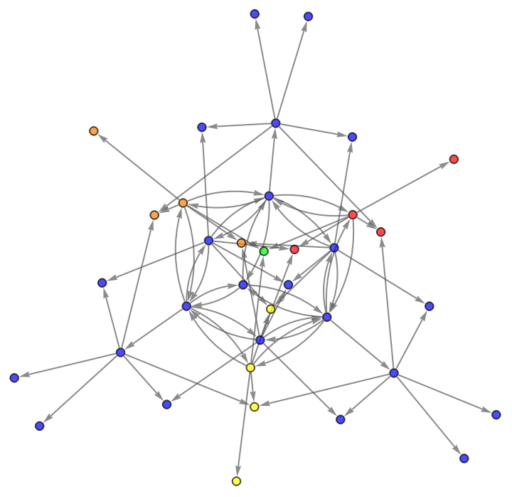
The vertex color in the reachability graphs indicates the entropy vector of the corresponding state, as we can observe,
EntropyHighlight[threeQubitStateGraph]
Out[]=
|


One useful measure of distance between pure quantum states in a Hilbert space is the Fubini-Study distance, defined =. The Fubini-Study distance between two states can be computed with the FSDistance[String1, String2] function, for example,
D
FS
1-ϕ,ψ
2
|
FSDistance[QuantumToString[{{1},{0},{0},{0},{0},{0},{0},{0}}],QuantumToString[{{1},{0},{0},{0},{0},{0},{0},{1}}]]FSDistance[QuantumToString[{{1},{1},{1},{1},{1},{1},{1},{1}}],QuantumToString[{{1},{0},{0},{0},{0},{0},{0},{1}}]]
Out[]=
1
2
Out[]=
3
2
Limitations on the maximal value of this graph velocity would indicate some “lightcone-type” structure that bounds the spread of information and entanglement in Branchial space. As we will find, the graph velocity never exceeds a maximal value of 1 for any explored qubit number and any quantum circuit.
Entanglement Multiway Graphs
Entanglement Multiway Graphs
In this section, we explore the propagation of information through multiway systems representing the evolution of physical systems through quantum circuits. Vertices in the multiway system state graphs represent different quantum states that have been reached during the evolution, and edges correspond to the quantum logic gates that transform states into others. Vertex color indicates the entropy vector, a description of entanglement structure, corresponding to that particular quantum state.
The sections below are organized according to the class of quantum circuit used to evolve each system. Systems evolved using only stabilizer circuits are accordingly labeled “Clifford evolution”. Those systems evolved using a quantum circuit with both Clifford and non-Clifford operations are indicated “Universal Evolution”.
The sections below are organized according to the class of quantum circuit used to evolve each system. Systems evolved using only stabilizer circuits are accordingly labeled “Clifford evolution”. Those systems evolved using a quantum circuit with both Clifford and non-Clifford operations are indicated “Universal Evolution”.
Building Multiway Graphs
Building Multiway Graphs
2-Qubits Clifford Evolution
2-Qubits Clifford Evolution
At two qubits the procedure is identical, though we now witness the arrival of multi-qubit gates such as the CNOT gate. We also have the potential for states to become entangled, with their entanglement structure indicated by the vertex coloration of the graph.
The full 2-qubit reachability graph can be constructed by assembling all 2-qubit stabilizer states and exploring their transformation on Clifford gate action.
However, we could also examine the evolution of a single state or some restricted subset of states, by initializing our multiway system to the restricted set. Below is the evolution of the 2-qubit vacuum under three steps through all stabilizer circuits.
It is possible, and sometimes quite useful, to generate three-dimensional renderings of graphs such as the above using Mathematica’s Graph3D function.
As with the single qubit systems, we can construct alternative representations of these multiway systems, such as the Branchial Graph, Event Branchial Graph, Causal Graph, and Layered Graphs.
4-Qubits Clifford Evolution
4-Qubits Clifford Evolution
While the 4-qubit rewriting rules can be explicitly regenerated from the code below, the computation time can get quite high. For this reason, I have made the 4-qubit rules data available for download here:
5-Qubits Universal Evolution
5-Qubits Universal Evolution
Computing Graph Velocities
Computing Graph Velocities
In this section, we compute and analyze Hilbert space and graph distances, and subsequently graph velocities for various graphs at increasing qubit number.
Clifford State Graph Velocities
Clifford State Graph Velocities
We begin by examining the stabilizer circuit evolution, plotting the Fubini-Study distance between all pairs of states against the reachability graph distance between those states. Below are the results for one, two, and three qubit systems.
We can likewise make a ListPlot of the non-duplicate velocity values encountered at one qubit. The minimal velocity value is zero, corresponding to gate action that maps a state to itself, while the maximum graph velocity is 1. The x-axis simply indicates the position of that particular velocity in the ordered list of values for the particular qubit number. As we increase the qubit number, more available velocities are found.
We could also generate the distribution of graph velocities for some collection of systems.
Finally, plotting graph velocities up through four qubits we have the following,
Discussion
Discussion
In this work, we examine systems of qubits evolved under a collection of quantum circuits. Circuits containing only Clifford operators, known as stabilizer circuits, always transform an initial state among some finite and discrete set of quantum states. Computing Hilbert space and graph space distances between states allows us to define some measure of velocity, describing how far a state can be moved in a Hilbert space under some number of applied quantum gates. We find that this velocity never exceeds 1, regardless of the quantum states being explored and the particular gates being applied. Furthermore, the possible velocities under Clifford group action form a discrete set with an interesting pattern that could be explored further. As we extend our analysis to include evolution by a universal gate set, we observe the same bound of graph velocity. We further observe the discrete set of attainable velocity values approaching some continuous curve. The distribution of velocities seems centered about lower values, seeming to indicate that smaller quantum circuits of local operations often result in small changes to a system.
References
References