Latin is a synthetic language; instead of relying on word order or extra helper words, it uses the contents of the words themselves to convey grammatical meaning. Hence, it has a free word order, meaning the same sentence can be expressed in different arrangements, all of which are grammatically valid. As a result, Latin syntax is, to some extent, ambiguous. In this computational essay, I model Latin syntax using context-free grammars (CFGs) and visualize possible derivations using Wolfram’s multiway systems to try to quantify the ambiguity potential of basic Latin phrases.
1 Introduction
1 Introduction
1.1 Context
1.1 Context
1.1.1 Context-Free Grammar
1.1.1 Context-Free Grammar
In formal language theory, a context-free grammar (CFG) is a formal grammar whose production rules can be applied to a non-terminal symbol regardless of its context. A production rule is a substitution rule. Below is an example of some production rules.
Creates a mini context-free grammar.
In[]:=
sampleCFG={{"A"}->{"B","C"},{"B"}->{"D"},{"D"}->{"C","A"}};
Production rules are made up of nonterminal and terminal symbols. A nonterminal symbol can be thought of as a placeholder or category. They need to be broken down further. In the production rules above, A, B, and D are all examples of nonterminal symbols. Terminals, on the other hand, cannot be broken down. Terminals are the end states of a CFG. In the example above, the only terminal is C because it does not map to any other letter.
If you start with a nonterminal state, the CFG will keep branching off until it reaches all terminal states. If a CFG does not contain a terminal state or set of terminal states, it will never resolve. Below is a representation of how graphs are formed step by step using the rules of the simple CFG .
Creates a slider for the step size of a multiway system using the mini context-free grammar that goes up to a max of 10.
In[]:=
Manipulate[ResourceFunction["MultiwaySystem"][sampleCFG,{"A"},x,"StatesGraph"],{x,0,10,1},SaveDefinitions->True]
Out[]=


1.1.2 Multiway Graphs
1.1.2 Multiway Graphs
A multiway graph is a graph representing all possible branches of evolution for a system. Each node in the graph represents a possible complete state of the system at a particular step, while each edge corresponds to the evolution of one state to another as a result of an updating event. In a causally invariant system, every branches in the multiway system must ultimately reconverge.
If a multiway system has a finite number of unique states (which is achieved depending on whether the rules it follows are restricting enough), it performs similarly to a finite-state automata (FSA). Finite-state automata, unlike CFGs, are used to sequentially process and parse text, particularly for regular languages, which are languages that are built upon regular expressions like “?”, “$”, and “\d.” On the other hand, multiway systems with rules that continue to expand to more states rather than converge to a certain set of them have infinite states.
If a multiway system has a finite number of unique states (which is achieved depending on whether the rules it follows are restricting enough), it performs similarly to a finite-state automata (FSA). Finite-state automata, unlike CFGs, are used to sequentially process and parse text, particularly for regular languages, which are languages that are built upon regular expressions like “?”, “$”, and “\d.” On the other hand, multiway systems with rules that continue to expand to more states rather than converge to a certain set of them have infinite states.
In formal language theory, when one uses CFGs to derive a sentence, the system is causally invariant. No matter which path you choose in the multi-way system, the paths converge perfectly on the exact same final string. However, parsing a string is not causally invariant, unless the grammar rules are completely unambiguous and deterministic.
1.1.3 Latin Syntax
1.1.3 Latin Syntax
The Chomsky hierarchy is a containment hierarchy (containing proper subsets) of classes of formal grammars. In this formal framework, Latin is classified as a Type-1 context-sensitive language. This is because it combines free words order with long distance, intersecting morphological agreements (case, gender, and number tracking). Free word order means we can scramble the words in a sentence and it would still make sense. Long-distance morphological agreements mean that words that belong together can be spaced far apart but still be linked together (e.g., matching suffix). Intersecting means these links can cross over each other like tangled threads. Since there is no “correct” word order, there are multiple ways you could arrange words within a sentence.
The three cells below translate a Latin sentence into English.
In[]:=
TextTranslation["Canis in via dormiebat","Latin"->"English"]
Out[]=
The dog was sleeping on the road.
In[]:=
TextTranslation["dormiebat in via Canis","Latin"->"English"]
Out[]=
The dog was sleeping on the road.
In[]:=
TextTranslation["via dormiebat Canis in","Latin"->"English"]
Out[]=
The dog was sleeping on the road.
However, this doesn’t mean that all word orders are applicable to express one idea. One famous example was given by the Delphic Oracle to Pyrrhus of Epirus before he fought the Romans.
“Aio te, Aecida, Romanos vincere posse.”
It can be translated as: “I say that you, descendant of Aeacus, are able to defeat the Romans.” But also: “I say that the Romans are able to defeat you, descendant of Aeacus.” Totally opposite meanings!
Pyrrhus took the first interpretation and went to war. Though he won the battles, he suffered such catastrophic losses that the term “Pyrrhic victory” was born.
1.2 Motivation and Research Question
1.2 Motivation and Research Question
While CFGs have been extensively used to analyze ambiguity in the field of computational linguistics, existing work relating such grammatical formulations to analyze the structural ambiguity of Classical Latin is surprisingly scanty. I believe that modeling Latin using CFGs could be a stepping stone towards connecting formal language theory to natural languages, especially for ambiguity analysis. CFGs offer a precise mathematical language for describing how sentences and phrases are built from smaller parts. By encoding Latin phrase structure as a CFG and tracing all valid derivations through a multiway system, one could quantify the number of ways that phrase can be parsed, and use it as a metric which can be manipulated and analyzed to identify ambiguity levels in Latin parsing. If such a metric is found, then it opens doors for computational analysis of Latin and potentially other syntactically similar natural languages.
For this project, my main goal was to analyze how syntactic ambiguity manifests in the parsing Classical Latin phrases via CFG derivations modeled using multiway systems, and to find out whether that ambiguity can be quantified and compared across different phrases.
1.3 Methodology
1.3 Methodology
The crux of my project lies in constructional homonymity: a property of certain strings of morphemes that have multiple syntactic interpretations given a singular structure and order. In the Latin language, a large chunk of these syntactic interpretations tend to result in the same meaning because of the free word order, but there are cases (e.g., Pyrrhus and the Delphic Oracle) where such interpretations do end up altering the meaning. Regardless, the higher the number of possible syntactic interpretations, the higher the number of potential ways to derive the original sentence. And so the number of possible parsing paths that lead to a phrase is a direct indicator of the ambiguity of the phrase, with fewer paths meaning less ambiguous and more paths meaning more ambiguous.
I decided that I would use the number of paths as my proxy for understanding Latin ambiguity in three ways:
1) Generating simple ambiguity percentages with the number of paths
2) Using the number of paths to create Bell number ratios of ambiguity
3) Using Shannon entropy to find the entropy of the path probabilities
To get the paths, I planned to create a CFG for the most common Latin phrases modeled off of the syntax presented on the Dickinson College website, which I would use as rules to create multiway graphs given some set of end terminals to find the number of paths it took to converge to the target nonterminal phrase type.
As for getting a dataset of Latin phrases to test on, I found a corpus of Latin phrases on Wikipedia and planned to pick out my own mini dataset from that list (with a size of at least 50 phrases).
2 Working Through a Simple Latin Noun Phrase
2 Working Through a Simple Latin Noun Phrase
To start off, I tested out making CFGs and multiway systems for a simple noun phrase: “magna urbs Romae.” Each word in the phrase can be classified as an adjective, noun, and noun, respectively. To keep track of the mapping between each word and its part of speech, I “tagged” each word with it’s part of speech. This is also known as PoS tagging, which is commonly used in NLP. I used PoS tagging to define the rules.
The input Latin sentence and its corresponding parts of speech.
In[]:=
nounPhrase="magna urbs Romae";tags={"ADJ","N","N"};
Because I was working with a simple phrase, I could use a basic, isolated form of a full context-free grammar list. For relevancy, this set of rules only applied to nouns, pronouns, and adjectives. To account for Latin’s free word order, all nonterminals which mapped to terminals of list size two or more had to have a supplemental palindromic form as well. For example, a nonterminal {“C”} which maps to {“A”,”B”} would also need to map to {“B”,”A”}.
Creating a list of rules for our basic noun phrase CFGs.
In[]:=
cfgNPBasic={{"NP"}->{"N"},{"NP"}->{"PRO"},{"NP"}->{"ADJ","NP"},{"NP"}->{"NP","ADJ"},{"NP"}->{"NP","NP"}};
Using a multiway system, I tested out the different graph structures which resulted from the basic CFG I had created for this phrase at various depth levels from an unspecific noun phrase state.
Defines a function which creates a multiway graph based on the basic noun phrase CFG for a given nonterminal state and step size. The graph object defaults to StatesGraph is no property argument is given.
In[]:=
forwardNPTree[x_List,y_Integer,z_String:"StatesGraph"]:=ResourceFunction["MultiwaySystem"][cfgNPBasic,x,y,z]
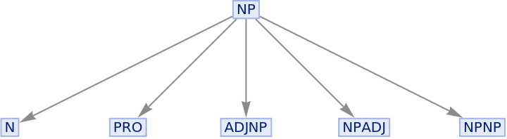
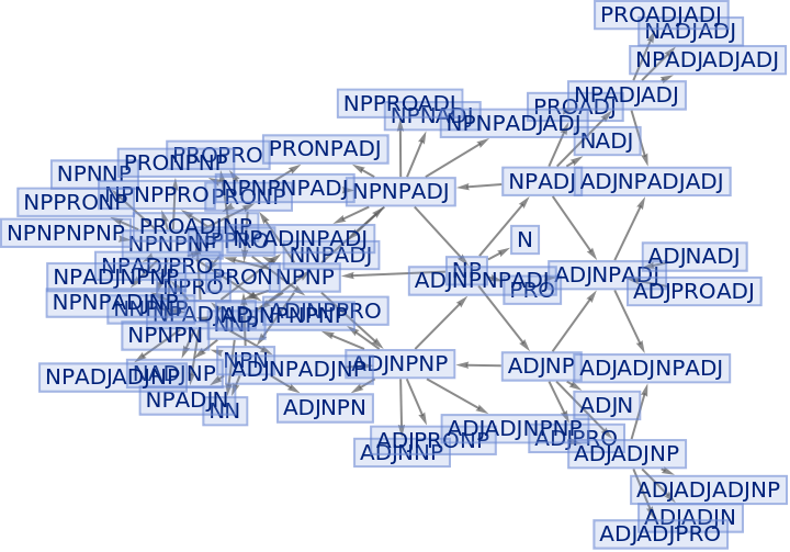
Creates three multiway graphs stemming from the {“NP”} state at step sizes one, three, and five (respectively)
In[]:=
forwardNPTree[{"NP"},1]forwardNPTree[{"NP"},3]forwardNPTree[{"NP"},5]
Out[]=
Out[]=
Out[]=
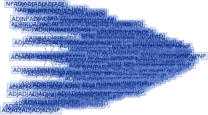
This forward multiway graph was an infinite-state automata (IFA), hence why it continued to grow as the step size increased.
Using Manipulate to create a slider for the step size from zero to five to see more clearly the evolution of the graph; the graph is set to StatesGraphStructure so that the nodes don’t cover the edges.
In[]:=
Manipulate[forwardNPTree[{"NP"},x,"StatesGraphStructure"],{x,0,5,1},SaveDefinitions->True]
Out[]=
The multiway I had made was a general case for any noun phrase that my basic CFG had accounted for. However, what I needed to find all possible parsing paths for “magna urbs Romae” specifically. Because I already knew the terminals of the phrase (“magna”, “urbs”, and “Romae”) and their tags (“ADJ”, “N”, “N”), I could work backwards to find all the possible ways to get from the terminals to the original noun phrase. Because I was reversing the parsing direction, I needed to reverse the basic CFG rules.
Map Reverse function to all entries in the basic CFG list to get inverse rules.
In[]:=
inverseCfgNP=Reverse/@cfgNPBasic
Out[]=
{{N}{NP},{PRO}{NP},{ADJ,NP}{NP},{NP,ADJ}{NP},{NP,NP}{NP}}
Then, I could plug the reversed CFG and the terminal tags into the same multiway system. Like before, I tested out a few graphs on the same phrase, increasing the number of steps for each one.
Defines a function identical to forwardNPTree except it builds off of the inverse CFG rules.
In[]:=
reverseNPTree[x_List,y_Integer,z_String:"StatesGraph"]:=ResourceFunction["MultiwaySystem"][inverseCfgNP,x,y,z]
Creates four multiway graphs stemming from a list of the terminal parts of speech of the input sentence at step sizes one, three, five, and seven (respectively)
In[]:=
reverseNPTree[tags,1]reverseNPTree[tags,3]reverseNPTree[tags,5]reverseNPTree[tags,7]
Out[]=
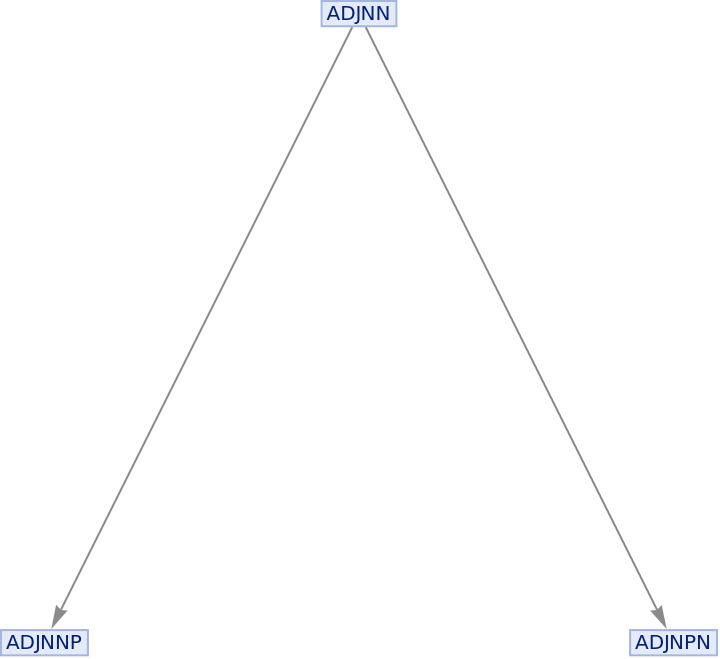
Unlike the forward multiway system, the reverse multiway system terminated at a state, so it was an FSA.
It seemed as though the graph had found all paths that lead to a noun phrase at either four or five steps. Using a slider, I could pinpoint that the step at which the graph stopped updating was at a step size of four.
Using Manipulate to create a slider for the step size from zero to five.
I visualized all of the possible event sequences using the “CausalGraphInstances” property, of which there were five distinct options.
Using CausalGraphInstances property of multiway systems to display all event sequences.
Now that I had this list, I tried to highlight these paths on the initial forward multiway graph that I had made earlier. I used the FindPath function to find all of the paths from the starting node and the last node.
Find all possible paths present in a reverse multiway system with step size four and input node of tags
Reversing the paths so that they are parsing in the same direction as the multiway state graph.
For reference, I first highlighted the shortest possible path between the terminals and the phrase, which I then compared with all of highlighted paths that I found on the reversed multiway graph.
Highlight the shortest path on the multiway state graph from the same starting and ending node.
Highlight the paths we got from the reversed multiway graph.
Having successfully extracted the number of paths, I had decided my general plan for path extraction moving forward: use my inverse CFG rule to create a multiway system to get the nonterminal phrase from the terminal parts of speech, extracting the paths as lists, and then reversing them back to original order.
3 Expanding to All Latin Phrases
3 Expanding to All Latin Phrases
Now that I had a general idea of how to set up CFGs and use them in multiway systems, I could expand the CFG list for all possible phrases that could come up in the Latin language. Just as I had done before, I had made all rules mapping to two or more states palindromic. Due to irregularities stemming from time period and stylistic quirks, these rules were broad enough to work for most typical phrase structure, but were not exhaustive by any means. One of the biggest challenges in this process was to determine how strict I would make the rules as to what constitutes the different types of phrases. For example, despite it being in the name, not all adverbial phrases have to contain adverbs in them. The same type of ambiguity exists for adjectival phrases. Technically, as long as the function as a whole “acts” like an adjectival or adverbial phrase, it can be considered one despite lacking an adjective or adverb, respectively. Because these distinctions were largely dependent on the other sentence elements, which I did not have access to, I needed to ignore those cases (except for a few outliers which were too commonly used for me to ignore).
Additionally, I needed to make sure that my rules were as concise as possible while still covering as many cases as possible. This was the hardest to do once I had added conjunctions as a potential terminal. Initially, I had only placed them in between two other terminals (e.g., “cat and dog”). However, I had neglected to account for phrases which start off with a conjunction (e.g., “because of the rain”). This required adding another case which lead with a conjunction. Because of my palindromic rule, I would then have to make a case which ended with a conjunction, even though I believed it to be rare if not nonexistent. As a result of this work, I would claim that my final Latin phrase CFG was generally broad enough to fit most cases, but by no means extensive or entirely essential.
In total, my final nonterminals were: noun phrase (NP), verb phrase (VP), adjectival phrase (ADJV), adverbial phrase (ADVP), prepositional phrase (PP), participial phrase (PARTP).
My terminals were: noun (N), verb (V), adjective (ADJ), adverb (ADV), preposition (P), participle (PARTP), conjunction (CONJ), infinitive (INF).
A rule list containing all CFGs mapping from the noun phrase nonterminal.
A rule list containing all CFGs mapping from the verbal phrase nonterminal .
A rule list containing all CFGs mapping from the adjectival phrase nonterminal; exception case: mapping directly to participial phrase.
A rule list containing all CFGs mapping from the adverbial phrase nonterminal; exception case: mapping directly to prepositional phrase.
A rule list containing all CFGs mapping from the prepositional phrase nonterminal.
A rule list containing all CFGs mapping from the participial phrase nonterminal.
Join rules lists for all phrase types to create full CFG.
Additionally, I created a few functions which would help me come up with parsing paths.
Two multiway graph functions which are identical except for the fact that one builds off of the regular CFGs (nonterminal to terminal(s)) and the other builds off the inverse CFGs (terminal(s) to nonterminal).
A function which returns a list of all the paths present in a reverseSystem graph.
The functions backTrack and findTruePaths work together to take a list of possible paths and return a list of paths which exist on both the forward and reverse system graphs. One thing I had taken for granted initially was that I had assumed two faulty things in my initial test with noun phrases:
1) The terminals would only converge to one state in the reverse multiway graph
1) All of the paths found in the reverse multiway graph would exist on the forward multiway graph
These were wrong assumptions. First of all, there is no rule forcing all terminals to branch to a pure nonterminal, much less the nonterminal which defines the type of phrase of the initial phrase. Because of the broadness of the CFG and its loops, it is possible for a phrase to branch to multiple different end states, which is a probability that gets larger as the phrase gets larger. Additionally, if all of the CFG rules were only one-way maps and were not palindromic and infinitely repeatable, then the second assumption would be true. However, that is not how the CFG is set up.
backTrack is a recursive function which checks to see if the children of the current node via multiway system with depth one, according to the forward CFG rule, contain the next node in a possible path. If the next node is not found within the list of possible outputs from the current node, then the recursion stops and returns false. If it is, then it continues looping until it has gone through all of the nodes in the path, at which point it returns true because all of the nodes in the path would’ve existed in the forward direction. Initially, I had simply generated a forward multiway graph , found all of the paths it had made to the terminals, looped through all of the possible parse paths, and checked to see which ones were in the list. While this method was technically possible, it was not efficient and caused the system to overload. A recursive function, which finds the child nodes from the parent node one step at a time, will have the same functionality and also prevent superfluous graphic generation.
A function which loops through the nodes of a possible path and recursively checks whether that path exists on the forward multiway system.
A function which cleans input paths of paths that don’t end at the correct nonterminal and calls backTrack to find whether these paths exist.
I could use the forwardSystem function to display the structures of the graphs for each type of phrase. I set my step size to three to avoid overloading the graphic output.
Creates six forward system StatesGraphStructure graphs at step size three for each type of noun phrase.
Notice how each graph appears to be vaguely symmetrical about an axis or set of axes? This is because of the palindromic nature of the CFGs. For every rule, there is an existing flip of that rule.
I also could use the findPossiblePaths and findTruePaths functions to return the total number of parses found by my CFG, as well as the number of parses which successfully traverse back to the correct nonterminal phrase state. I tested this out with the phrase “divisa in partes tres”, where the target nonterminal phrase state would be a participial phrase.
Makes a slider for the step size of the reverseSystem which up to seven because beyond seven the graph stops updating
Find the number of parseable paths and the number of paths from that list of parseable paths which correctly maps to the original phrase state.
It was imperative for me to keep track of both the possible number of paths and the actual number of paths, since they introduced another metric by which I could analyze the ambiguity of phrases: parses which map to the correct nonterminal phrase, and parses which map to that nonterminal phrase along with the other possible constructions my current CFG allowed.
4 Ambiguity
4 Ambiguity
There is no widely-accepted or standard way to determine the ambiguity of language, so my analysis had to be done comparatively. Consequently, I made a corpus of phrases to pull from, containing the sentence and PoS tags. I conducted all statistics on this list of 54 phrases and compared my results against each phrase in this corpus to get an understanding of ambiguity distribution amongst common Latin phrases.
Corpus of noun phrases with appropriate PoS tags.
Corpus of verb phrases with appropriate PoS tags.
Corpus of prepositional phrases with appropriate PoS tags.
Corpus of adverbial phrases with appropriate PoS tags.
Corpus of adjectival phrases with appropriate PoS tags.
Corpus of participial phrases with appropriate PoS tags.
Corpus of all phrases joined together.
4.1 Basic Ambiguity Metrics
4.1 Basic Ambiguity Metrics
Perhaps the simplest way to calculate ambiguity is to calculate the percentage of phrases which have more than one possible way to parse them out of the whole corpus of phrases. For example, if only one phrase out of the group has one possible parse path, then the ambiguity percentage would be low. If almost all of the phrases in a group have more than one parse path, then the ambiguity percentage would be high.
I decided that I wanted to compare my data within two separate scopes. First, I wanted to be able to compare all phrase-specific data with the rest of the entire corpus. Secondly, I wanted to be able to group those stats into categories based on the type of phrase they were, and then compare those phrase groupings together. With this in mind, I needed to have access to the phrase, its classification, and its respective PoS tag. Additionally, as I mentioned in section two, for each phrase, I wanted to be able to access both all of the possible parsings as well as all of the parsing which match the phrase type (i.e., the “true” parsings). To begin, I needed to collate and store my data in such a way that I would have access to all information necessary to perform this analysis.
Gathers data from the entire corpus and formats to create nested lists containing phrase type, phrase, and PoS tag.
Takes information from the corpus to find all possible parsings for each phrase as well as all true parsings for each phrase using functions created in section 3; stores nested lists containing type of phrase, phrase, and list of paths found.
Finds length number of paths found for both possible and true path conditions; stores nested lists containing type of phrase, phrase, and number of paths found.
Once I had collated all of the necessary data to perform the analysis, I decided to measure three simple metrics: ambiguity percentage, the mean number of parses per phrase, and the maximum number of parses recorded for a phrase. First, so that I had a global baseline of these metrics, I calculated them within the context of the entire corpus.
A function which extracts either the mean number of parsings, the max number of parsings, or the ambiguity percentage from a list of derivations.
Baseline ambiguity percents for derivations containing all possible paths and true paths.
Baseline mean for derivations containing all possible paths and true paths.
Baseline max for derivations containing all possible paths and true paths.
Next, I needed to be able to group the same metrics by phrase type. I ended up using an association for this task, where the keys were the phrase types and the value was another association, which contained the metrics as keys, including an additional metric to keep count of number of phrases, all mapping to the initial state of zero.
List of all types of noun phrases in the corpus.
Two associations for each type of phrase, containing associations storing the number of phrases (“count”), the ambiguity percent, the mean number of parses, and the maximum number of parses: one for storing data for derivations containing all possible paths, the other for storing data for derivations containing true paths.
The associations were updated by passing them and their respective derivation list into a function which looped through each value. Except for the max metric, the ambiguity percentage and mean metrics after the updates needed to be divided by the value of the count metric to get the final values.
A function which loops through derivation lists to update the stats of its respective association.
Updated stats for both derivation lists after passing through updatedStats function.
Once all of the values had been updated, I created one bar chart for each association displaying the ambiguity percentage of each phrase type.
Creates bar charts for both stats associations grouped by phrase type.
Additionally, I wanted to see how the max and mean metrics related to each other, so I gathered the metric lists from both associations and plotted them onto a scatterplot to see how they related to each other across all types of phrases.
Gets the max parse number from each stats association per type of phrase.
Gets the mean parse number from each stats association per type of phrase.
Creates a scatterplot of mean and max lists from both associations.
Although these metrics were good to have as a baseline, they were too rudimentary and random to have much of any useful information regarding the ambiguity of Latin phrase syntax. This was especially true given the sparseness and lack of diversity within the Latin phrase corpus I used to come up with these values.
4.2 Bell Number Ratios
4.2 Bell Number Ratios
To be able to quantify the relative ambiguity of a phrase in Latin, it might be preferable to create a scale such that a number close to zero would represent an unambiguous parse and a number close to one would represent a maximally ambiguous parse. One could try to normalize to this scale by dividing the number of possible parses of a phrase in Latin by the maximum number of possible parses of that phrase in any language (whether or not that maximally ambiguous language exists!). To calculate this latter number, consider the collection of words A, B, and C.
The collection can be parsed as the terminals A, B, and C all combined into a single nonterminal: (ABC).
The terminals A, B, and C could also form singleton nonterminals that combine into the top-level nonterminal: (A)(B)(C).
The collection can also be parsed as any one terminal combined with an intermediate nonterminal element formed from the other two terminals: e.g., (A)(BC).
Because each word must be part of a grouping, but there is no constraint on the size of that grouping, one can generalize that the maximum number of parses for a phrase with a given set of words can be approximated by the number of ways to partition a set containing the same number of elements into subsets. This is known as the Bell number and can be computed using Wolfram’s BellB function. I decided to use this function to create another ambiguity metric, where instead of calculating an ambiguity percentage, I get a ratio where I would divide the number of parsings by the Bell number to get a list of ratios, which I then would normalize to be on a scale between zero and one.
A function which extracts the information from a derivations list relevant for doing Bell number analysis; stores nested lists containing type of phrase, phrase, the word count of the phrase, and the number of parsings.
Lists containing the Bell numbers for both derivation lists in the structure set up by the bellNumberAnalysis function.
I decided to visualize the two ambiguity ratio lists as two histograms to see how the value distribution changed between all possible paths and true paths.
A function which calculates the ambiguity ratio by dividing the number of parsings of a phrase by the Bell number of the word count of that phrase, then rescales to a value between 0 and 1.
List of ambiguity ratios extracted from both derivation lists.
Creates histograms for ambiguity ratios of both derivation lists.
4.3 Shannon Entropy
4.3 Shannon Entropy
One might try to seek a more probability based analysis to determine ambiguity. It is known that high probabilities signify likely events, while low probabilities signify unlikely events. If this is applied to parsing, the higher the probability of a parsing path, the more likely it will be used. For example, phrases with only one parse path have al 100% chance of being used, while phrases with seven parse paths each have around a 14.3% chance of being used. Since ambiguity increases as the number of parse paths increases, one can make the conclusion that the certainty or uncertainty of a path can be used to determine whether a path is unambiguous or ambiguous, respectively. Thus, entropy is a valid ambiguity metric. I decided to use Shannon Entropy, a mathematical measure of the average entropy given a probability distribution, to determine the uncertainty levels of the phrases in my corpus.
I assumed that the probability of each was equally likely (i.e., the probability of each path is equal to 1/n, where n is the total number of paths), and calculated the Shannon entropy of each probability list for each phrase to get a list of entropy values. The assumption that all parses are equally likely results in a relationship between the number of possible parses and the entropy that is simple to reason about.
Let n be the number of possible parses. Plugging 1/n directly into each probability term, the formula for entropy becomes:
All terms inside the summation are now independent from the summation index and can be extracted by multiplying by n:
Finally, the standard logarithmic simplification rule applies:
A function which extracts the information from a derivations list relevant for calculating Shannon entropy; stores nested lists containing type of phrase and a list of all of the probabilities for each parse path.
Lists containing the entropy values for both derivation lists in the structure set up by the getProbs function.
A function which calculates the Shannon entropy of a list of probabilities.
List of entropy values from both probability lists.
I decided to visualize the two entropy value lists as two histograms the same way I visualized the bell ratio values so that I could compare the two results.
Creates histograms for entropy values of both probability lists.
Analysis
Analysis
Although the ambiguity metrics presented in section 4.1 weren’t enough to draw solid conclusions about ambiguity of Latin as a whole, the bar charts do highly represent the ambiguity present in each phrase type’s CFGs. For example, the fact that nearly all of the phrase groups had a 100% ambiguity rate intuitively makes sense since I’ve classified any number of possible parses greater than one makes a phrase ambiguous. When you include all types of paths without sifting them for specific states, the probability of a phrase to have more than one possible parse increases rapidly. As for the second bar chart, what struck my eye at once was the low ambiguity percentage of participial phrases. In the corpus, nine out of the 10 participial phrases have PoS tags like {“PART”} and {“N”, “PART”}, and the CFGs for participial phrases don’t allow for starting states like the ones in the corpus to map very far. According to the CFG, the only thing {“PART”} can map to is itself, and for {“N”, “PART”}, first {“N”} will map to a noun phrase, and then it becomes {“NP”, “PART”}, which maps back to the participial phrase. So, shallow CFG rules with little depth result in lower ambiguities. Adjectival phrases had the highest ambiguity percentage for the direct opposite reason: the CFGs for adjectival phrases map to multiple other kinds of states (e.g., noun phrases, prepositional phrases, participial phrases, etc.). Additionally, despite there being a smaller number of adjectival phrases in the corpus, their PoS are more diverse and varied than those for the participial phrases.
I also want to take some time to address the outlier on the scatterplot: the phrase which had 895 possible parses. That phrase was the participial phrase “divisa in partes tres.” The reason why this phrase had so many parses is because each PoS maps to a different phrase CFG. The phrase contains a participle, a preposition, a noun, and an adjective, making it an incredibly diverse sentence.
However, moving onto Bell ratio and Shannon entropy, I noticed an interesting behavior that I believe reveals some information about the ambiguity of Latin phrase syntax. As a convenient unit for the structural ambiguity of a Latin phrase, I introduce the notion of an ambiguity potential, i.e. the additional ambiguity in meaning imparted by the addition of a single word. As discussed above in section 4.3, the entropy simply scales logarithmically with the number of possible parses, and is thus agnostic to phrase length, unlike the Bell number ratio, discussed in section 4.2. The Bell number scales monotonically with its argument, the number of words in the phrase, so the Bell number ratio decreases as the phrase length increases, if the number of possible parses is fixed. Given two phrases, where one is longer than the other but both have the same number of valid parsings, the Bell ambiguity will be lower than the entropy for the longer phrase because the same number of parses are being divided by the larger Bell number, while the log is being taken of the same number for the entropy. Even if the longer phrase has slightly more parsings, which still indicates a low ambiguity potential because those extra words didn’t add much more ambiguity, the Bell number might be lower for the longer phrase, while the entropy would be higher! Comparing the first histogram in sections 4.2 and 4.3, the entropy value for my corpus was vaguely gaussian, centered around some intermediate number, but the Bell distribution had its peak at zero and quickly tailed off. It is clear that the corpus if full of cases where the entropy shows more ambiguity than the Bell ratio, which happens when longer phrases have similar or only slightly larger ambiguity than shorter phrases. Thus, the ambiguity potential is low in a synthetic language like Latin!
Limitations and Further Directions
Limitations and Further Directions
I believe that the biggest limitation of this project was the lack of centralized data surrounding Latin syntax. Because I didn’t have access to a list of common grammatical structures and orders of parts of speech, I had to come up with them myself, and although I believe they were accurate enough to execute this project somewhat decently, the results would certainly have been clearer and more accurate if such a list existed. In a similar vein, I had to create my own corpus of phrases and tag all of their parts of speech using my own prior knowledge and the online Latin dictionary William Whitaker’s Words (William Whitaker’s Words, n.d.). As a result, there could be human errors in my work, and each phrase type didn’t have the same number of phrases per category. That last part especially could have skewed the data represented in the bar charts in section 4.1.
There are a lot of directions where this work can lead. One potential avenue could be to extend the scope and to look at whole Latin sentences rather than Latin phrases: something which I would’ve wanted to do if I had more time. Another avenue could be to analyze ambiguity by mapping paths around the “head” of a Latin phrase or sentence to determine whether its position can influence what kind of orientation the words have around it. On that note, one could replicate my Shannon entropy analysis, but instead of assigning the probabilities of n paths to each be 1/n, they could try to find probabilities that skew more towards paths that have a recorded property that increases the likelihood of that path being picked (e.g., having the shortest path length or a popular structure in the historical period the phrase was written). Of course, this same analysis could be applied and modified to fit other languages as well.
Conclusion
Conclusion
In this computational essay, I have constructed and analyzed a CFG for Latin phrase syntax, encoding the language’s free word order through palindromic production rules and visualizing the resulting derivations using multiway systems. Applying this grammar to a corpus of 54 manually tagged Latin phrases, I computed two complementary ambiguity metrics:
1) Bell number ratios, which measured parse count relative to a theoretical maximum
2) Shannon entropy, which measured average uncertainty over parse paths under a uniform probability assumption.
Analysis of the Bell number and Shannon entropy histograms both converged on the same conclusion that Latin phrase syntax, even when modelled as a context-free language that permits all word-order permutations, exhibits low structural ambiguity. This finding supports a potential hypothesis that morphology effectively constrains interpretive ambiguity even without fixed word order. The framework developed here is readily extensible to full sentences rather than phrases, to other synthetic languages such as Ancient Greek or Sanskrit, or even to analytic languages such as English or Mandarin for comparative study.
Acknowledgements
Acknowledgements
This project would not have been possible without the guidance of my mentor CJ, who helped outline the process for me and always listened to me talk about how I debugged some niche error even when she never asked. Thank you to TAs Eric and Kaaya for helping me debug and optimize my code, my dorm mates Sreeja, Rachel, Jolie, Gaurika, Meher, and Saanvi for the emotional support and frantic late-night coding hangouts, TA Amrita for always coming up to our dorm when we were too lazy to go down for check-in, and program directors Rory, Eryn, Megan, and Cyrus for making this experience enjoyable for everyone.
Additional thanks to Stephen Wolfram for suggesting this project
Additional thanks to Stephen Wolfram for suggesting this project
References
References
1
.Anand, N. (n.d.). [WSRP23] Exploring computational dynamics of formal-language syntax using multiway systems. Wolfram Community. https://community.wolfram.com/groups/-/m/t/2965584
2
.Asked ChatGPT to pick 10 random phrases from each letter section of the Wikipedia phrase data
3
.Ayer, M. (n.d.). Important Rules of Syntax. Dickinson College Commentaries. Retrieved July 9, 2026, from https://dcc.dickinson.edu/grammar/latin/important-rules-syntax
4
.Bell Number. (n.d.). Wolfram MathWorld. https://mathworld.wolfram.com/BellNumber.html
5
.Bell’s Numbers and the Bell Triangle: Significance and Derivation. (n.d.). Statistics How To. Retrieved July 9, 2026, from https://www.statisticshowto.com/bells-numbers-bell-triangle/
6
.Causal Invariance -- from Wolfram MathWorld. (n.d.). Wolfram MathWorld. Retrieved July 9, 2026, from https://mathworld.wolfram.com/CausalInvariance.html
7
.Chomsky, N. (2015). Syntactic Structures. Martino Fine Books.
8
. Context-Free Grammars [College slideshow describing CFGs] [PDF]. (n.d.). Stanford.
9
.Gorard, J., Wolfram, S., & Piskunov, M. (n.d.). MultiwaySystem. Wolfram Function Repository. https://resources.wolframcloud.com/FunctionRepository/resources/MultiwaySystem
10
.Hockenmaier, J. (n.d.). Lecture 2: Finite-state methods for morphology [UIUC Lecture on FSAs]. In Lecture 2. University of Illinois Urbana-Champaign.
11
.Kharbouch, A., & Karam, Z. (n.d.). Three Models for the Description of Language. 6.
12
.List of Latin phrases (full). (n.d.). Wikipedia. Retrieved July 9, 2026, from https://en.wikipedia.org/wiki/List_of_Latin_phrases_(full)
13
.Multiway System -- from Wolfram MathWorld. (n.d.). Wolfram MathWorld. Retrieved July 9, 2026, from https://mathworld.wolfram.com/MultiwaySystem.html
14
.POS(Parts-Of-Speech) Tagging in NLP. (2026, July 2). GeeksforGeeks. Retrieved July 9, 2026, from https://www.geeksforgeeks.org/nlp/nlp-part-of-speech-default-tagging/
15
.Prasad, G. (2025). [WSRP25] Unambiguity properties in context-free grammars: identifying a maximal unambiguous rule set. Wolfram Community. https://community.wolfram.com/groups/-/m/t/3499683
16
.SHANNON’S THEOREM. (n.d.). University of Pennsylvania, 6.
17
.What is Context-Free Grammar? (2025, July 23). GeeksforGeeks. Retrieved July 9, 2026, from https://www.geeksforgeeks.org/theory-of-computation/what-is-context-free-grammar/
18
.William Whitaker’s Words. (n.d.). Archives of the University of Notre Dame. Retrieved July 9, 2026, from https://archives.nd.edu/words.html
CITE THIS NOTEBOOK
CITE THIS NOTEBOOK
Using context-free grammars and multiway systems to analyze the ambiguity of Latin syntax
by Smriti Siva
Wolfram Community, STAFF PICKS, July 9, 2026
https://community.wolfram.com/groups/-/m/t/3754144
by Smriti Siva
Wolfram Community, STAFF PICKS, July 9, 2026
https://community.wolfram.com/groups/-/m/t/3754144