Motivation: Integer Precision
Motivation: Integer Precision
One of the greatest achievements of modern physics is its powerful use of symmetry. At the human scale, symmetries abound: by simple experimentation as children we find that the laws of our natural world are unaffected by translations, rotations, and the passage of time. These are global symmetries, and they correspond to invariant quantities, the familiar conservation laws which determine so many natural phenomena.
As we study physics at higher energy scales, revealing the particle foundations of nature, these symmetries largely persist -- but we also begin to observe new, stricter symmetries. These symmetries require that physics be invariant under transformations of local “gauge” degrees of freedom, which occur independently at each point in spacetime. Three of the fundamental forces of nature (the exception, as always, being gravity) have been modelled with incredible precision by gauge theories, where the local degrees of freedom are represented by certain well-known Lie groups.
Despite our limited understanding of the properties which a unified quantum theory of gravity should fulfill, many physicists have come to strongly suspect that the continuous nature of spacetime is an approximation which breaks down at the Planck scale. If this hypothesis holds, a quantum theory of gravity must describe dynamics with some discretized model, whose continuum limit reproduces both the Standard Model of particle physics and General Relativity.
The aim of this project is to study how local gauge symmetries may be represented by undirected graphs, as motivated by the hypergraph-replacement models for fundamental physics proposed in [1]. We use the language of fibre bundles to build an intuition for the characteristics of gauge theories which must be present in our models, and demonstrate familiar physical features of the resultant bundle graphs for U(1) electromagnetism on. While gauge theories built upon discrete networks are well-studied, and form the basis of lattice gauge theory, there has been significantly less investigation of entirely discrete models, where the gauge group itself is not permitted to be continuous. In a sense we are returning to a world of integers, where the only meaningful quantities are counts of network connections, with well-founded hope that the complexities of our physical world will be fully describable.
As we study physics at higher energy scales, revealing the particle foundations of nature, these symmetries largely persist -- but we also begin to observe new, stricter symmetries. These symmetries require that physics be invariant under transformations of local “gauge” degrees of freedom, which occur independently at each point in spacetime. Three of the fundamental forces of nature (the exception, as always, being gravity) have been modelled with incredible precision by gauge theories, where the local degrees of freedom are represented by certain well-known Lie groups.
Despite our limited understanding of the properties which a unified quantum theory of gravity should fulfill, many physicists have come to strongly suspect that the continuous nature of spacetime is an approximation which breaks down at the Planck scale. If this hypothesis holds, a quantum theory of gravity must describe dynamics with some discretized model, whose continuum limit reproduces both the Standard Model of particle physics and General Relativity.
The aim of this project is to study how local gauge symmetries may be represented by undirected graphs, as motivated by the hypergraph-replacement models for fundamental physics proposed in [1]. We use the language of fibre bundles to build an intuition for the characteristics of gauge theories which must be present in our models, and demonstrate familiar physical features of the resultant bundle graphs for U(1) electromagnetism on
3
Background: Fibre Bundles
Background: Fibre Bundles
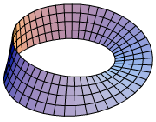
The usual intuition for defining a fibre bundle is a topological space which is everywhere locally equivalent to the product of a base space and fibre space, respectively, but which globally need not be a trivial product. Formally the bundle is defined by a continuous surjection , which satisfies the property that it may be locally inverted onto the product space . A familiar non-trivial example is the Möbius strip, which may be constructed by “fibreing” an interval over circle -- locally, we could not tell this object from a cylinder, but clearly it has a global topology which is distinct and contains a twist.An essential construct on a fibre bundle for our purposes is the connection. Since each point in the base space has a unique fibre, if we want to compare data on one fibre with another nearby, we must identify a correspondence between them. This process, known as parallel transport, emerges similarly in general relativity, where parallel transport describes how vectors and reference frames transform along a curve in curved spacetime. In a gauge theory, “curvature” emerges from the choice of a connection, and ultimately defines the configuration of a gauge field. Therefore we may think of the connection as a rule which, given any infinitesimal path through spacetime B, returns an infinitesimal path through the entire bundle space E.When we move to a discrete structure, any path through our base graph consists of a sequence of links between vertices. In order to define a connection in this same language, it is apparent that the entire bundle must also be describable by a graph , where the connection is a link-lifting map . We will see that this identification has clear consequences for the connectivity of and its physical interpretation. In a gauge theory, since the fibres of the bundle are copies of gauge group G (this is referred to as a principal G-bundle), we can think of local gauge invariance as the requirement that physical observables are invariant under all diffeomorphisms which only map each fibre onto itself.
E
BxF
π:EB
BxF
[0,1]⊂
1
S
Δx
Δe
G
B
G
E
C:E[]E[]
G
B
G
E
G
E
EE
Demonstration: Discrete Hopf U(1)-Bundle
Demonstration: Discrete Hopf U(1)-Bundle
As an illustrative example, we turn to the work of Manton [3], who studied the problem of discrete gauge theories in the topologically non-trivial example of a Hopf bundle. Manton makes use of a 24-vertex regular 4D polytope as an approximation to the manifold , which will be shown to have a reducible structure. The result will be a discrete analogue of the Hopf bundle, a fibre bundle with where each fibre is a copy of the group .
3
S
E=,B=
3
S
2
S
U(1)
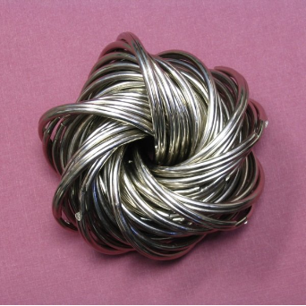
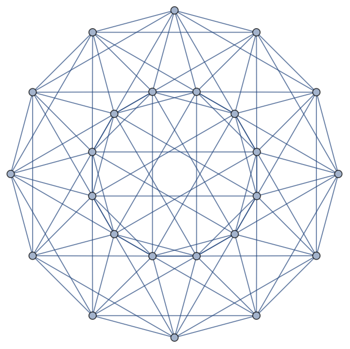
Any 2D or 3D projection of this polytope is necessarily limited in scope, and blurs the symmetry of the object. Fortunately, from graph connectedness alone, it is possible to understand this symmetry: all vertices have identical local linkedness and global positioning, as should be expected from rotational invariance.
A specific labelling scheme for these vertices is chosen in [3] which aids in understanding their connectedness. Embedding coordinates in are reduced to , with eight vertices chosen to lie at the extrema of the two real and two imaginary axes. These eight vertices provide a tiling of by 16 spherical triangles -- the remaining vertices are placed at the centers of these. Each vertex has eight nearest neighbors, represented by edges in the figure above.
4
2
3
S
Out[]=
{{0,1},{0,},{0,-1},{0,-},{1,0},{,0},{-1,0},{-,0},{1+,1+},{1+,1-},{1+,-1-},{1+,-1+},{1-,1+},{1-,1-},{1-,-1-},{1-,-1+},{-1-,1+},{-1-,1-},{-1-,-1-},{-1-,-1+},{-1+,1+},{-1+,1-},{-1+,-1-},{-1+,-1+}}
The edge connectivity under this labelling scheme was entered by hand to confirm various minor results in [3], and confirmed to produce a graph isomorphic to the 24-polytope native to Mathematica. With this labelling, an immediate pattern is visible -- for every vertex , also appears in the graph. We therefore have six independent group orbits of four vertices each, which can be labelled by the invariant quantity . The six invariants can then be said to index the fibres of the (soon-to-be) bundle, and will be identified by the following color scheme:
V={a,b}
V={a,b}
Z=a·
-1
b
{0,∞,1,,-1,-}
{0,∞,1,,-1,-}
,,,,,


We choose to add edges to the graph which visually identify the group orbits -- it is important to note that vertices are not otherwise connected within each fibre, as no information necessary for calculation is gained. The true edges between fibres are colored in white. Several key features are identifiable by eye, once we establish the procedure of selecting a gauge. Since each fibre in the bundle corresponds to a single point on our (octahedral) spacetime manifold, a dynamical closed-loop path need not begin and end at the same vertex in bundle space. Instead, we may consider any path which begins on a vertex of a given color and ends on a vertex of that same color. Following the example in [3], we might consider loops around the = sequence of fibres. Eight such loops exist, three of which begin and end on the same vertex in bundle space -- these three paths are said to have a holonomy of 0, while the others have holonomies corresponding to the group elements . Fixing a gauge for the entire bundle is equivalent to selecting an edge in fibre space for every pair of adjacent fibres. As detailed in [3], each fibre in this bundle has four adjacent fibres, for a total of 12 edges in the base space -- and every fibre vertex has two neighboring vertices on each adjacent fibre . Therefore, even for this small structure, a staggering possible connections exist, representing the quantity of allowed dynamical configurations.
{∞,1,,∞}
,,,
{,-1,-}
12
2
Construction: Are We Braiding? (or are we dancer)
Construction: Are We Braiding? (or are we dancer)
With this example in mind, we proceed to constructing fibre bundles on a more general space: a lattice in which will serve as the base space of our gauge theory.
n
Building U(1)-Bundles on Lattices
Building U(1)-Bundles on Lattices
In this example we consider a d=3 lattice graph with size 5 in each dimension. We will demonstrate how to build a discrete U(1)-bundle on this lattice base space, using the cyclic group as a finite approximation.
C
6
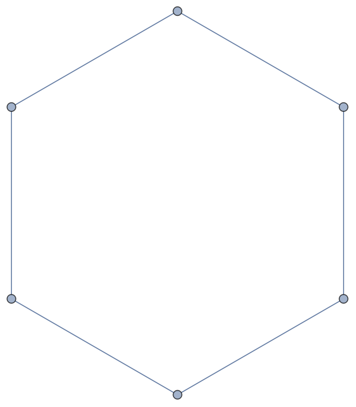
As explained in [4], the key quantities in a lattice gauge theory are the parallel transport operators which indicate how the gauge group action is communicated between neighboring lattice sites. These operators take values from G (as opposed to the continue case where they live in the Lie algebra of G). By assigning an element of G to each edge of our base graph, we therefore totally define the gauge field configuration.
With this bundle construction, key physical quantities acquire clear translations. Permutation group representations appear as braidings (although these graphs do not know about their own knottedness). Parallel transport along any vertex path is simply the composition of braidings, giving a total gauge action for the path in question, and Wilson loops may easily be defined. We first confirm that Wilson loops sum appropriately, such that they are an extensive property of the base space.
With this phase equivalence, we can more easily examine additivity of Wilson loops, and confirm the functionality of our plaquette function, which computes the smallest possible Wilson loop taking a given vertex as the top-left corner.
We may think of any Wilson loop or plaquette as indicating the magnetic flux across its (oriented) subtended surface [5]. The 1st Chern number in this setting quantifies the total emanating flux from a volume -- we expect this to be 0 for any choice of connection due to topological triviality of this bundle / existence of a global section. This is confirmed below for every unit volume in the lattice.
Dynamics: A New Hope
Dynamics: A New Hope
To further investigate this, we set a flat connection, which contains zero magnetic charge.
On the same plaquette P = 32-37-38-33-32, we can instead achieve a total of six twists while restricting ourselves to only make single or double twists on each edge. No plaquettes experience phase ambiguity, and the result is a dipole operator over the two unit volumes bordering P. We may envision a unit string of flux which crosses P but terminates on both ends before crossing any other plaquettes.
Many more simple operators for perturbing a flat connection can likely be constructed, and are an essential tool for exploring the dynamics of this model.
Conclusions and Future Directions
Conclusions and Future Directions
The construction of a discrete analogue of a U(1) gauge theory is a significant step in attempting to model fundamental particle physics with graphs and hypergraphs. This work has succeeded in showing how local gauge invariance can manifest purely from connectedness data -- however, there is much work still to be done. Even in this relatively simply model, we have observed anomalies which depend upon our choice of phase interpretation of the discrete gauge group. Exploring the consequences for dynamics in the model will be key, and in order to fully approach that challenge, we must gain a clearer understanding of how evolution must proceed in order to respect the local gauge symmetry. Subgraph-replacement dynamics for hypergraphs as put forward in have already been shown to carry local symmetries forward on each time step under the right circumstances [1, 6.12 and 8.19], and so a possible avenue is to design replacement rules which perform similar operations to the flux and monopole operators described in the previous section. We would further like to extend the construction here to non-Abelian gauge groups including SU(2) and SU(3), which is hoped to be largely straightforward as long as sufficient simple permutation representations of discrete approximations to these groups may be found.
Acknowledgments
Acknowledgments
Mentor: Kiel Howe
I am deeply grateful for all the help and guidance I received from my project mentor Kiel Howe, Jonathan Gorard, Stephen Wolfram, Tali Beynon, Andoni Royo, and the entire WSS 2020 team for supporting this research!
References
References
◼
[1] Wolfram Physics Project: Technical Documentation. https://www.wolframphysics.org/technical-introduction/
◼
[2] A.M. Turing. Approximations to Lie Groups. Ann. Math. 39 (1938), no. 1, 105--111.
◼
[3] Manton, N. S. Connections on discrete fibre bundles. Comm. Math. Phys. 113 (1987), no. 2, 341--351. https://projecteuclid.org/euclid.cmp/1104160217
◼
[4] Tong, D. Gauge Theory. Lecture Notes. https://www.imperial.ac.uk/media/imperial-college/research-centres-and-groups/theoretical-physics/msc/dissertations/2014/Nicholas-Prouse-Dissertation.pdf
◼
[5] Prouse, N.W. Magnetic Monopoles in Pure Compact Lattice Quantum Electrodynamics. Thesis, Imperial College London. https://www.imperial.ac.uk/media/imperial-college/research-centres-and-groups/theoretical-physics/msc/dissertations/2014/Nicholas-Prouse-Dissertation.pdf
CITE THIS NOTEBOOK
CITE THIS NOTEBOOK
Full Discretization of Local Gauge Invariance
by Graham Van Goffrier
Wolfram Community, STAFF PICKS, July 14, 2020
https://community.wolfram.com/groups/-/m/t/2030337
by Graham Van Goffrier
Wolfram Community, STAFF PICKS, July 14, 2020
https://community.wolfram.com/groups/-/m/t/2030337