The Wolfram quantum framework integrates with standard computational analysis and modeling tools, enabling symbolic quantum computations, numerical measurement-based quantum computing, and interaction with quantum hardware. A recent addition to the framework is the Suzuki-Trotter decomposition, known as Trotterization, which simulates quantum time evolution in circuits. This computational essay briefly reviews Trotterization within the framework and demonstrates its application through examples, showcasing its utility in modeling quantum systems.
Paclet installation
Paclet installation
Install quantum paclet (to add quantum functions to WL):
In[]:=
PacletInstall["https://wolfr.am/DevWQCF",ForceVersionInstall->True]<<Wolfram`QuantumFramework`
Out[]=
PacletObject

In[]:=
Names["*Quantum*"]
Out[]=
{QuantumBasis,QuantumChannel,QuantumCircuitMultiwayCausalGraph,QuantumCircuitMultiwayGraph,QuantumCircuitOperator,QuantumDistance,QuantumEntangledQ,QuantumEntanglementMonotone,QuantumEvolve,QuantumMeasurement,QuantumMeasurementOperator,QuantumMeasurementSimulation,QuantumMPO,QuantumMPS,QuantumOperator,QuantumPartialTrace,QuantumPartialTranspose,QuantumShortcut,QuantumState,QuantumStateEstimate,QuantumStateEstimation,QuantumStateSampler,QuantumTensorProduct,QuantumWeylTransform,QuantumWignerTransform}
Time evolution and Trotterization
Time evolution and Trotterization
Consider a simple Ising-type of Hamiltonian for three qubits as with X/Z Pauli operators:
H=++--
X
1
X
2
X
3
Z
1
Z
2
Z
2
Z
3
In[]:=
h=QuantumOperator["X"+("X"->{2})+("X"->{3})-"ZZ"-("ZZ"->{2,3})];
The decomposition into Pauli matrices:
In[]:=
h["PauliDecompose"]
Out[]=
XII1,ZZI-1,IXI1,IZZ-1,IIX1
Also, the Hamiltonian can be constructed differently:
In[]:=
h==Sum[QuantumOperator["X",{i}],{i,3}]-Total[QuantumOperator["ZZ",#]&/@Partition[Range[3],2,1]]
Out[]=
True
Find time-dependent state:
In[]:=
ψt=QuantumEvolve[h,{t,0,10}];
Plot bit-string probabilities in time:
In[]:=
ListAnimate[BarChart[#,ChartLabels->StringJoin@@@Tuples[{"0","1"},3],PlotRange->{-.1,1}]&/@Table[ψt["Probabilities"],{t,0,10,.1}]]
Out[]=
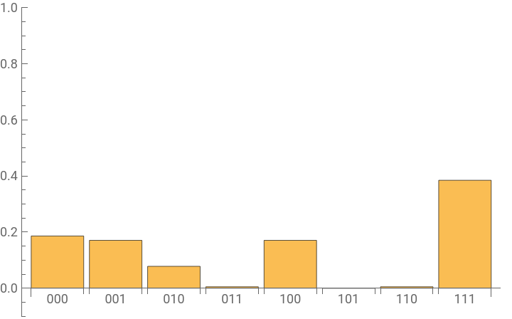
Now let’s explore how a circuit can mimic the above time evolution. The goal is to create a quantum circuit, approximating the time evolution operator. For the simple case of time-independent Hamiltonian, it means a circuit mimicking Exp[- t H], to some approximation. Assuming , the exponential product formula (ie the Suzuki-Trotter decomposition) will be very useful.
H=
∑
i
A
i
Trotterization can be implemented in our framework as follows:
where ListOfOperators are in fact the list of operators constructing the Hamiltonian, and OrderOfApproximation represents the order corrections to the exponential product formula.
QuantumCircuitOperator[{"Trotterization",ListOfOperators,OrderOfApproximation,NumerOfSteps,OverallTime}]
where ListOfOperators are in fact the list of operators constructing the Hamiltonian, and OrderOfApproximation represents the order corrections to the exponential product formula.
List of Pauli operators where h=Total[ops] (note it is useful to do so because here the operator h depends only on Pauli operators)
In[]:=
ops=KeyValueMap[QuantumOperator[#2#1]&,h["PauliDecompose"]];
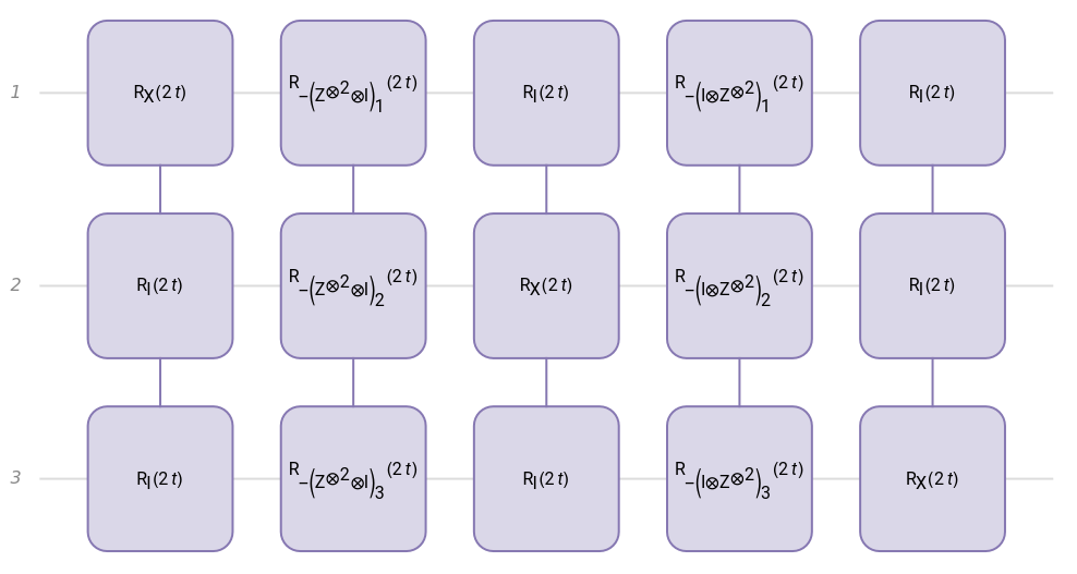
Trotter-Suzuki decomposition of first order and one step:
In[]:=
QuantumCircuitOperator[{"Trotterization",ops,1,1,t}]["Diagram",FontSize->8]
Out[]=
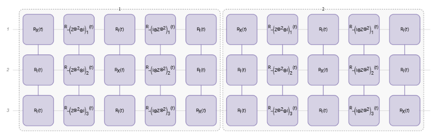
Trotter-Suzuki decomposition of first order and two steps:
In[]:=
QuantumCircuitOperator[{"Trotterization",ops,1,2,t}]["Diagram",FontSize->8]
Out[]=
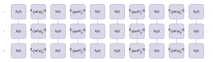
Trotter-Suzuki decomposition of 2nd order and one step:
In[]:=
QuantumCircuitOperator[{"Trotterization",ops,2,1,t}]["Diagram"]
Out[]=
Trotter-Suzuki decomposition of 2nd order and two steps:
In[]:=
QuantumCircuitOperator[{"Trotterization",ops,2,2,t}]["Diagram",FontSize->6]
Out[]=

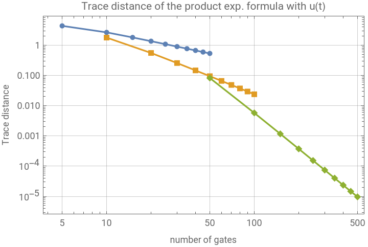
Calculate the trace distance between the evolution operator at time with the one obtained from the Troterrization (to do so, I will use QuantumDistance, but we should wrap the operator matrices as QuantumState, first, to feed it into QuantumDistance) :
t=1
In[]:=
u=MatrixExp[-h["Matrix"]];//AbsoluteTiming
Out[]=
{16.1191,Null}
In[]:=
uf=QuantumState[u];
In[]:=
tracDis=Table[With[{c=N[QuantumCircuitOperator[{"Trotterization",N@ops,order,steps,1}]]},{c["Gates"],QuantumDistance[QuantumState[c["Matrix"]],uf,"Trace"]}],{order,{1,2,4}},{steps,1,10}];//AbsoluteTiming
Out[]=
{300.097,Null}
Visualize it:
In[]:=
ListLogLogPlottracDis,
Out[]=


Another metric one can use to test how good the Trotterization approximate the actual evolution operator is the spectral norm (which is Norm[...,2] in Wolfram Language).
In[]:=
norm2=Table[With[{c=N[QuantumCircuitOperator[{"Trotterization",N@ops,order,steps,1}]]},{c["Gates"],Norm[c["Matrix"]-u,2]}],{order,{1,2,4}},{steps,1,10}];//AbsoluteTiming
CITE THIS NOTEBOOK
CITE THIS NOTEBOOK
Suziki-Trotter decomposition: simulating Hamiltonian dynamics
by Mads Bahrami
Wolfram Community, STAFF PICKS, NOV 7, 2022
https://community.wolfram.com/groups/-/m/t/2687830
by Mads Bahrami
Wolfram Community, STAFF PICKS, NOV 7, 2022
https://community.wolfram.com/groups/-/m/t/2687830