Creating a collection of examples involving both definite and indefinite integrals is an excellent approach to comprehensively understand and illustrate the concepts of integration in calculusThis collection would be a valuable resource for students and educators alike, providing a comprehensive look at integration in calculus through a wide range of examples.
Indefinite integral
Indefinite integral
Indefinite Integrals are the integrals that can be calculated by the reverse process of differentiation and are referred to as the antiderivatives of functions . For a function , if the derivative is represented by (x), the integration of the resultant (x) gives back the initial function .
F(x)
′
f
′
f
F(x)
∫f(x)dxF(x)+C
◼
′
F
◼
C
In the above definition :
◼
f(x)
◼
dx
x
◼
F(x)
In[]:=
Integrate[f[x],x]
Out[]=
∫f[x]x
Important Formulas of Indefinite Integrals
Important Formulas of Indefinite Integrals
In[]:=
Integrate[1,x,GeneratedParameters->C]
Out[]=
x+
1
In[]:=
Integrate[e^x,x,GeneratedParameters->C]
Out[]=
1
x
e
Log[e]
In[]:=
Integrate[x^n,x,GeneratedParameters->C]
Out[]=
1+n
x
1+n
1
In[]:=
Integrate[1/x,x,GeneratedParameters->C]
Out[]=
1
In[]:=
Integrate[Cos[x],x,GeneratedParameters->C]
Out[]=
1
In[]:=
Integrate[Sin[x],x,GeneratedParameters->C]
Out[]=
1
In[]:=
Integrate[a^x,x,GeneratedParameters->C]
Out[]=
1
x
a
Log[a]
In[]:=
Integrate[1/Sin[x]^2,x,GeneratedParameters->C]
Out[]=
1
In[]:=
Integrate[1/Cos[x]^2,x,GeneratedParameters->C]
Out[]=
1
Calculate the indefinite Integrals
Calculate the indefinite Integrals
◼
∫(+cosx+sinx)dx
3
x
In[]:=
Integrate[x^3+Cos[x]+Sin[x],x,GeneratedParameters->C]
Out[]=
4
x
4
1
◼
+x+1dx
2
x
x
In[]:=
Integrate[(x^2+x+1)/x,x,GeneratedParameters->C]
Out[]=
x+++Log[x]
2
x
2
1
◼
+8dx
3
x
x+2
In[]:=
Integrate+8,x,GeneratedParameters->C
3
x
x+2
Out[]=
4x-++
2
x
3
x
3
1
◼
∫tanxdx
In[]:=
Integrate[Tan[x],x,GeneratedParameters->C]
Out[]=
1
◼
sin2x+dx
π
6
In[]:=
Integrate[Sin[2x+Pi/6],x,GeneratedParameters->C]
Out[]=
1
1
2
π
6
Definite Integrals
Definite Integrals
The definite integral of a function is closely related to the antiderivative and indefinite integral of a function
b
∫
a
◼
The integrand
f(x)
◼
The integral bounds and , where is the lower bound and is the upper bound. These are also referred to as limits.
a
b
a
b
◼
The differential , which tells us that we are integrating with respect to the variable .
dx
f
x
Definite Integrals vs . Indefinite Integrals
Definite Integrals vs . Indefinite Integrals
It' s important to understand the difference between definite and indefinite integrals .
Finding the indefinite integral and finding the definite integral are operations that output different things .
1
.Calculating the indefinite integral takes in one function, and outputs another function
2
.Definite integrals find the area between a function' s curve and the on a specific interval.
x-axis
How to Calculate Definite Integrals
How to Calculate Definite Integrals
The value of the definite integral of a function on is the difference of any antiderivative of the function evaluated at the upper limit of integration minus the same antiderivative evaluated at the lower limit of integration.
[a,b]
We can use the Fundamental Theorem of Calculus :
If is continuous and is an antiderivative of , then
If
f
F
f
b
∫
a
Examples
Examples
1
.Let' s calculate 3dx
6
∫
2
In[]:=
Integrate[3,{x,2,6}]
Out[]=
12
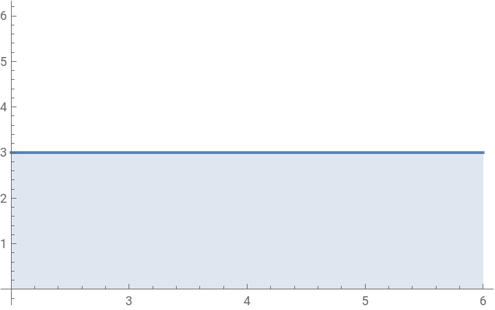
Visualize the area given by this integral :
In[]:=
Plot[3,{x,2,6},Filling->Axis]
Out[]=
2
.Let’ s calculate 4-2xdx
2
∫
1
3
x
In[]:=
Integrate[4x^3-2x,{x,1,2}]
Out[]=
12
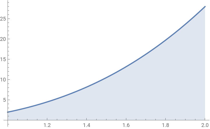
In[]:=
Plot[4x^3-2x,{x,1,2},Filling->Axis]
Out[]=