This notebook implements a custom Particle Swarm Optimization (PSO) algorithm in Mathematica and benchmarks it against the Rastrigin function, a classic non-convex test function known for its many regularly spaced local minima that make it a challenging target for optimization algorithms. Two versions of the objective are defined: a standard 4-dimensional Rastrigin function with global minimum at the origin, and a constrained variant that adds a penalty term forcing the solution onto (or near) the unit hypersphere. Before running PSO, both problems are solved using Mathematica’s built-in NMinimize with the Differential Evolution method. The obtained solutions are to be used to validate the PSO results.
The PSO implementation itself is built from modular helper functions: clipMatrix and clampMatrix enforce position and velocity bounds column-wise, while the core psoOptimize function handles swarm initialization, velocity updates using inertia weight and cognitive/social acceleration coefficients (c1, c2), and iterative tracking of personal-best and global-best positions and scores. The swarm uses linearly decaying inertia weight across iterations, random uniform coefficients for exploration/exploitation balance, and velocity clamping as a fraction of the search range to prevent divergence. Progress is logged every 10 iterations, printing the current best loss value.
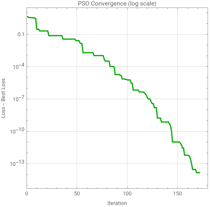
For the unconstrained Rastrigin test, the swarm of 30 particles converges rapidly, driving the loss from roughly 0.29 down to numerical zero within about 170–180 iterations, closely matching the known global minimum near the origin found by NMinimize. A log-scale convergence plot of the “gap” (current loss minus best-known loss) shows a characteristic staircase pattern, reflecting the swarm escaping successive local minima before settling into the global basin.
For the constrained variant, the penalty term pushes the swarm toward solutions satisfying x1²+x2²+x3²+x4²≈1, and the algorithm converges more slowly, taking roughly 150–160 iterations to reach a stable loss near 1.0, consistent with the reference solution from NMinimize. The corresponding convergence plot again shows a stair-step descent on a log scale, though with a longer plateau early on, reflecting the added difficulty of simultaneously satisfying the spherical constraint while minimizing the underlying multimodal Rastrigin landscape.
In[]:=
Rastrigin[x_List]:=10*Length[x]+Sum[x[[i]]^2-10*Cos[2*Pi*x[[i]]],{i,Length[x]}];
Constrained variant:force solution onto/near the unit hypersphere
RastriginConstrained[{x1_,x2_,x3_,x4_}]:=Rastrigin[{x1,x2,x3,x4}]+10^6*(x1^2+x2^2+x3^2+x4^2-1)^2;
In[]:=
sol4=NMinimize[{Rastrigin[{x1,x2,x3,x4}],-5.12<=x1<=5.12,-5.12<=x2<=5.12,-5.12<=x3<=5.12,-5.12<=x4<=5.12},{x1,x2,x3,x4},Method->"DifferentialEvolution",AccuracyGoal->20,PrecisionGoal->20]
Out[]=
{0.,{x1-3.39554×,x2-2.73625×,x3-2.58261×,x4-5.30476×}}
-11
10
-12
10
-11
10
-12
10
In[]:=
sol4Constrained=NMinimize[{Rastrigin[{x1,x2,x3,x4}],x1^2+x2^2+x3^2+x4^2==1,x4>0.1},{x1,x2,x3,x4},Method->"DifferentialEvolution",AccuracyGoal->20,PrecisionGoal->20]
Out[]=
{1.,{x1-7.20715×,x2-7.26347×,x3-7.65548×,x41.}}
-9
10
-9
10
-9
10
Upper and lower bounds for the search domain
FitnessLB=-{5,5,0.2,5};FitnessUB={5,5,1.2,5};
PSO parameters
c1=1.42;c2=1.42;w=0.72984;
SeedRandom[42];
4D problem
SwarmDim=4
Out[]=
4
PSO code
Clip each COLUMN of a matrix against its own scalar bound
clipMatrix[mat_,lbv_,ubv_]:=Transpose[MapThread[Clip[#1,{#2,#3}]&,{Transpose[mat],lbv,ubv}]];clampMatrix[mat_,vmaxv_]:=Transpose[MapThread[Clip[#1,{-#2,#2}]&,{Transpose[mat],vmaxv}]];
PSO Optimizer
psoOptimize[lossFunc_,dim_,lb_,ub_,nParticles_:30,nIter_:100,wMax_:0.9,wMin_:0.4,c1_:1.42,c2_:1.42,vClampFrac_:0.2]:=Module[{particles,velocities,pbest,pbestScore,gbest,gbestScore,convergence={},r1,r2,scores,gbestIdx,vmax,wIter},vmax=vClampFrac*(ub-lb);particles=Transpose@Table[RandomReal[{lb[[i]],ub[[i]]},nParticles],{i,dim}];velocities=ConstantArray[0.,{nParticles,dim}];pbest=particles;pbestScore=lossFunc/@particles;gbestIdx=First@Ordering[pbestScore,1];gbestScore=pbestScore[[gbestIdx]];gbest=pbest[[gbestIdx]];Do[wIter=wMax-(wMax-wMin)*(j-1)/(nIter-1);r1=RandomReal[1,{nParticles,dim}];r2=RandomReal[1,{nParticles,dim}];velocities=wIter*velocities+c1*r1*(pbest-particles)+c2*r2*(ConstantArray[gbest,nParticles]-particles);velocities=clampMatrix[velocities,vmax];particles+=velocities;particles=clipMatrix[particles,lb,ub];scores=lossFunc/@particles;pbest=MapThread[If[#3<#2,#1,#4]&,{particles,pbestScore,scores,pbest}];pbestScore=MapThread[Min,{pbestScore,scores}];gbestIdx=First@Ordering[pbestScore,1];If[pbestScore[[gbestIdx]]<gbestScore,gbestScore=pbestScore[[gbestIdx]];gbest=pbest[[gbestIdx]];];AppendTo[convergence,gbestScore];If[Mod[j,10]==0,Print["PSO Iter ",j," Loss = ",gbestScore]];,{j,nIter}];{gbest,gbestScore,convergence}];
unconstrained Rastrigin test function
In[]:=
Fitness1[{x1_,x2_,x3_,x4_}]:=Rastrigin[{x1,x2,x3,x4}]
PSO run
result1=psoOptimize[Fitness1,SwarmDim,FitnessLB,FitnessUB,1000,300];{gbest1,gbestScore1,convergence1}=result1;
PSO Iter 10 Loss = 0.287637
PSO Iter 20 Loss = 0.19966
PSO Iter 30 Loss = 0.0729754
PSO Iter 40 Loss = 0.035088
PSO Iter 50 Loss = 0.0252175
PSO Iter 60 Loss = 0.00192615
PSO Iter 70 Loss = 0.00103993
PSO Iter 80 Loss = 0.000316038
PSO Iter 90 Loss = 0.0000180973
PSO Iter 100 Loss = 5.72654×
-6
10
PSO Iter 110 Loss = 6.56708×
-7
10
PSO Iter 120 Loss = 1.31891×
-7
10
PSO Iter 130 Loss = 1.67712×
-9
10
PSO Iter 140 Loss = 7.14458×
-10
10
PSO Iter 150 Loss = 1.00755×
-11
10
PSO Iter 160 Loss = 6.03961×
-13
10
PSO Iter 170 Loss = 1.42109×
-14
10
PSO Iter 180 Loss = 0.
PSO Iter 190 Loss = 0.
PSO Iter 200 Loss = 0.
PSO Iter 210 Loss = 0.
PSO Iter 220 Loss = 0.
PSO Iter 230 Loss = 0.
PSO Iter 240 Loss = 0.
PSO Iter 250 Loss = 0.
PSO Iter 260 Loss = 0.
PSO Iter 270 Loss = 0.
PSO Iter 280 Loss = 0.
PSO Iter 290 Loss = 0.
PSO Iter 300 Loss = 0.
In[]:=
gbest1
Out[]=
{-2.83485×,1.61916×,-1.7415×,3.64558×}
-9
10
-9
10
-9
10
-10
10
Gap to the best-known solution at each iteration
gap=convergence1-gbestScore1;ListLogPlot[gap,Joined->True,PlotRange->{{0,180},Automatic},Frame->True,FrameLabel->{"Iteration","Loss - Best Loss"},PlotLabel->"PSO Convergence (log scale)",PlotStyle->Darker@Green,AspectRatio->1,GridLines->Automatic]
Out[]=
constrained Rastrigin test function
In[]:=
Fitness2[{x1_,x2_,x3_,x4_}]:=RastriginConstrained[{x1,x2,x3,x4}]
PSO run
result=psoOptimize[Fitness2,SwarmDim,FitnessLB,FitnessUB,1000,300];{gbest,gbestScore,convergence}=result;
PSO Iter 10 Loss = 26.4736
PSO Iter 20 Loss = 12.3991
PSO Iter 30 Loss = 12.3015
PSO Iter 40 Loss = 12.3015
PSO Iter 50 Loss = 11.4912
PSO Iter 60 Loss = 11.4912
PSO Iter 70 Loss = 8.91102
PSO Iter 80 Loss = 8.27937
PSO Iter 90 Loss = 8.27277
PSO Iter 100 Loss = 8.02631
PSO Iter 110 Loss = 5.59196
PSO Iter 120 Loss = 1.05917
PSO Iter 130 Loss = 1.01047
PSO Iter 140 Loss = 1.0001
PSO Iter 150 Loss = 1.00001
Gap to the best-known solution at each iteration
CITE THIS NOTEBOOK
CITE THIS NOTEBOOK
PSO for constrained and unconstrained Rastrigin function minimization
by Housam Binous
Wolfram Community, STAFF PICKS, July 3, 2026
https://community.wolfram.com/groups/-/m/t/3743678
by Housam Binous
Wolfram Community, STAFF PICKS, July 3, 2026
https://community.wolfram.com/groups/-/m/t/3743678