This notebook (which generously borrows from Robert Rimmer's notebook here) pulls data from a website for United States data, put together by a group at The Atlantic. The site tracks testing that has been performed as well as the number of positive tests, which seem to follow well the cases reported by JHU CSSE. The full dataset is updated each day between 4pm and 5pm EDT, with limited updates as new information arrives. The data used here seem to be lagging behind slightly relative to the data at Worldometers.
In[]:=
usDailyTracking=Import["https://covidtracking.com/api/us/daily","RawJSON"]/.NullMissing[]//Dataset;
Convert to Mathematica dates and plot raw data.
Out[]=
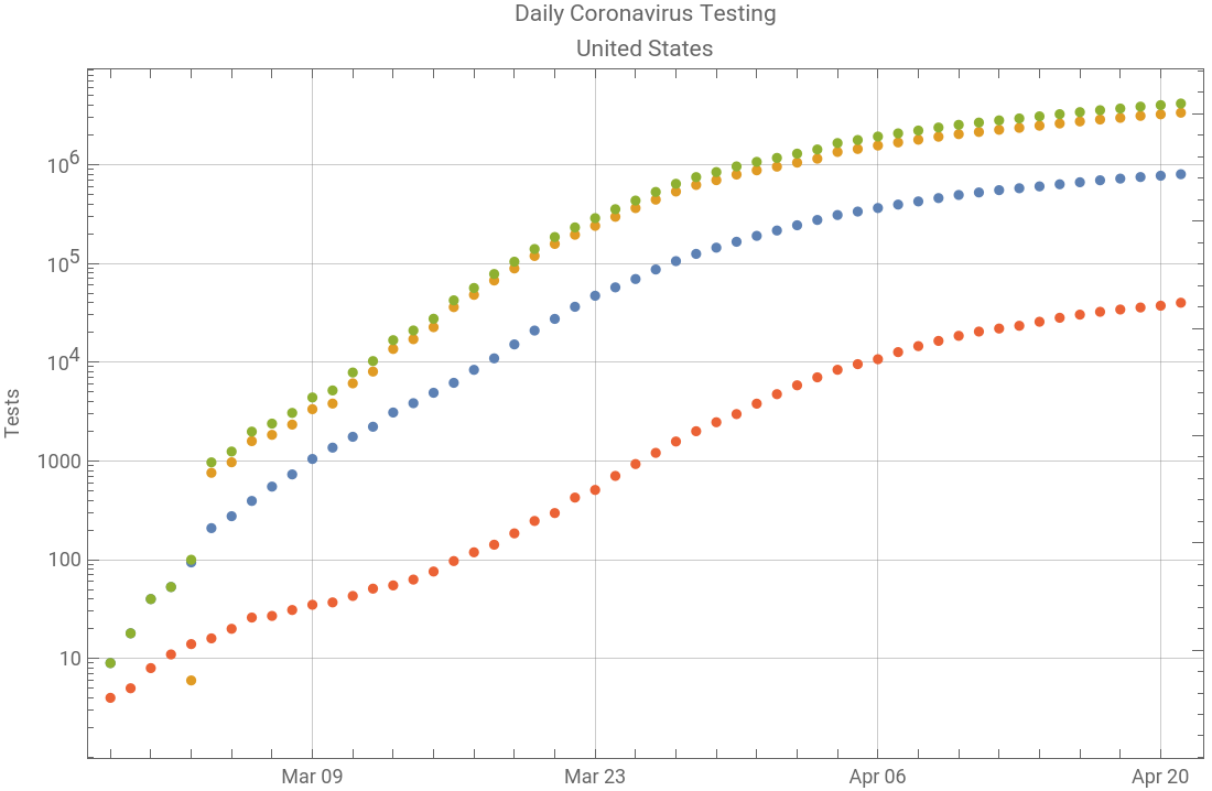


We’re pulling out some data for later analysis.
In[]:=
posData=Reverse@usDaily[All,{"date","positive"}]//Normal//Values;posDataMA=Transpose@Join[{posData〚7;;,1〛},{MovingAverage[posData〚All,2〛,7]}];dailyPosMA=Transpose@Join[{posData〚8;;,1〛},{Differences[posDataMA〚All,2〛]}];deadData=Reverse@usDaily[All,{"date","death"}]//Normal//Values;deadDataMA=Transpose@Join[{deadData〚7;;,1〛},{MovingAverage[deadData〚All,2〛,7]}];dailyDeadMA=Transpose@Join[{deadData〚8;;,1〛},{Differences[deadDataMA〚All,2〛]}];
Logistic Function fitting
In[]:=
epidemicDates[NLM_FittedModel]:=DatePlus{2020,1,21},Floort0-/.NLM@"BestFitParameters",DatePlus{2020,1,21},Ceilingt0+/.NLM@"BestFitParameters";Clear[differenceLogReport];differenceLogReport[cases0_List,opts___]:=Module{nlm,cases,dates,MPB95},If[Head[cases0[[1]][[1]]]===DateObject,cases=Transpose[{DateDifference[{2020,1,21},#][[1]]&/@cases0[[All,1]],cases0[[All,2]]}],If[Head[cases0[[1]][[1]]]===Integer,cases=cases0,Return[]]];Print@cases[[-1]];nlm=NonlinearModelFitcases,,{{k,0.3},{L,cases[[-1]][[2]]},{t0,cases[[-1]][[1]]}},t;MPB95=nlm["MeanPredictionBands",ConfidenceLevel.95];Print[nlm@"BestFitParameters"];dates=epidemicDates[nlm];dtlist=DateRange[DatePlus[{2020,1,21},cases[[2]][[1]]],dates[[2]]];Print@DateListPlot[{Tooltip[#,#]&/@Transpose[{dtlist,Differences@Log[nlm[#]&/@Range[cases[[1]][[1]],DateDifference[{2020,1,21},dates[[2]]][[1]]]]}],Tooltip[#,#]&/@Transpose[{Take[dtlist,Length@cases-1],Differences@Log@N@cases[[All,2]]}]},opts,JoinedFalse,FrameTrue,FrameLabel{None,"Daily Growth Rate"},PlotLegends{"Predicted","Actual"},GridLinesAutomatic,ImageSize600];{nlm,TimeSeries[cases],dates,MPB95};LogFunFitModel[cases0_List]:=Module{nlm,cases,dates,MPB95},If[Head[cases0[[1]][[1]]]===DateObject,cases=Transpose[{DateDifference[{2020,1,21},#][[1]]&/@cases0[[All,1]],cases0[[All,2]]}],If[Head[cases0[[1]][[1]]]===Integer,cases=cases0,Return[]]];nlm=NonlinearModelFitcases,,{{k,0.3},{L,cases[[-1]][[2]]},{t0,cases[[-1]][[1]]}},t,MaxIterations1000;MPB95=nlm["MeanPredictionBands",ConfidenceLevel.95];dates=epidemicDates[nlm];{nlm,TimeSeries[cases],dates,MPB95};ResLogFunModel[cases_,n_]:=Module[{nn},nn=If[n≤Length[cases],n,Length[cases]];LogFunFitModel[cases[[Table[i,{i,1,nn}],All]]]];
Log[-1+L]
k
Log[-1+L]
k
L
1+
-k(t-t0)
L
1+
-k(t-t0)
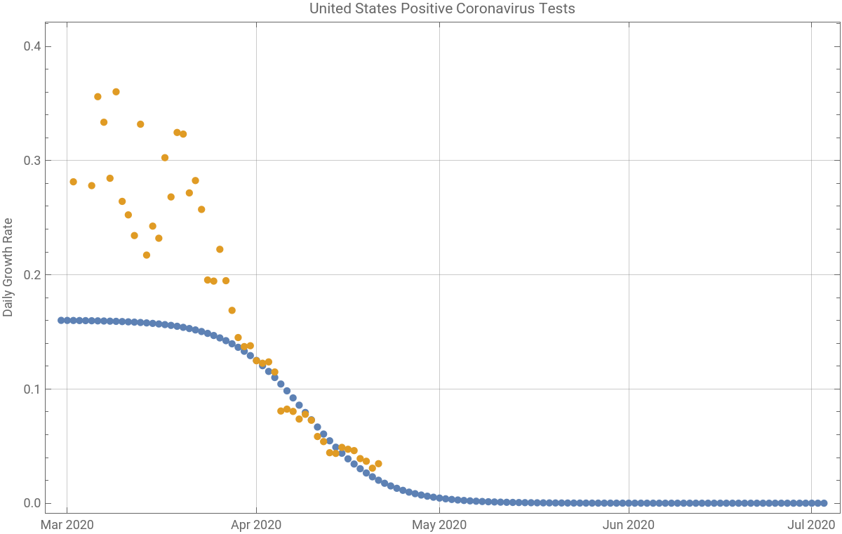
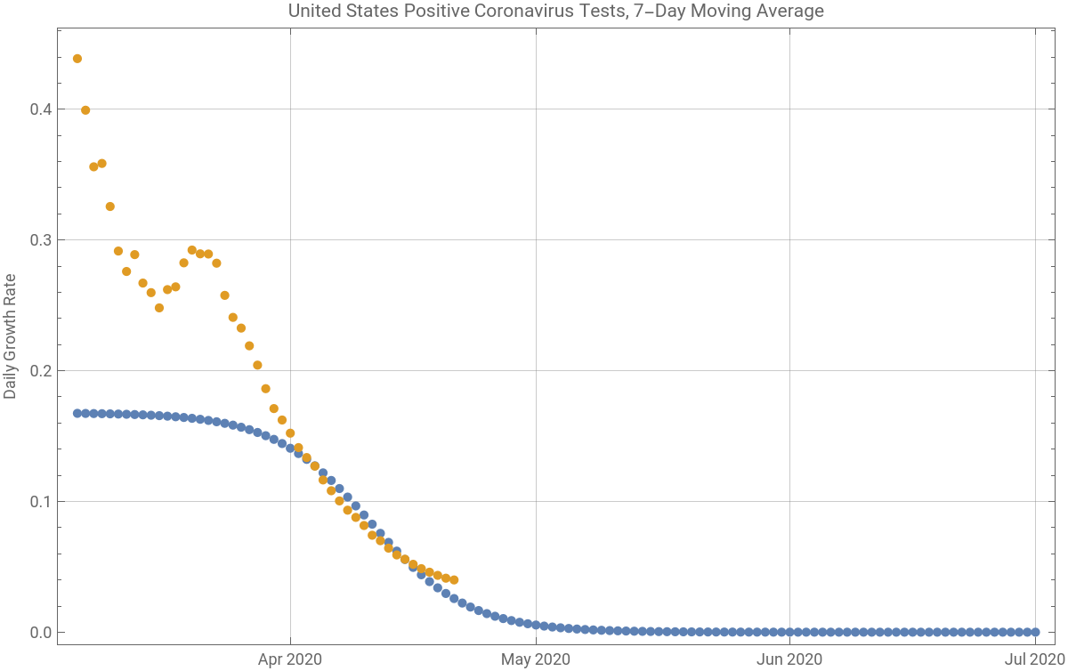
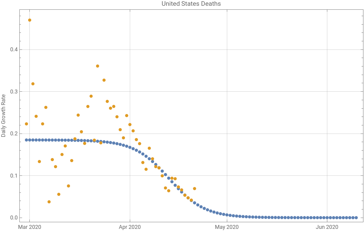
The graphics below provide one perspective for tracking the epidemic. The orange points are the daily differences of the logarithm of accumulated cases, i.e. an estimate of the continuous growth rate of the number of cases. The blue dots are the predicted daily rates for the course of the epidemic by a logistic growth model constrained by quarantine. The logistic model parameters are estimated from the accumulated data at the last orange point.
In[]:=
posmodel=differenceLogReport[posData,PlotLabel"United States Positive Coronavirus Tests"];posmodelMA=differenceLogReport[posDataMA,PlotLabel"United States Positive Coronavirus Tests, 7-Day Moving Average"];
{91,799717}
{k0.160352,L876056.,t078.3835}
91,
5034062
7
{k0.167822,L815020.,t080.3163}
In[]:=
deadmodel=differenceLogReport[deadData,PlotLabel"United States Deaths"];deadmodelMA=differenceLogReport[deadDataMA,PlotLabel"United States Deaths, 7-Day Moving Average"];
{91,39995}
{k0.184868,L47168.8,t082.687}
91,
238069
7
{k0.192517,L42986.8,t084.5706}
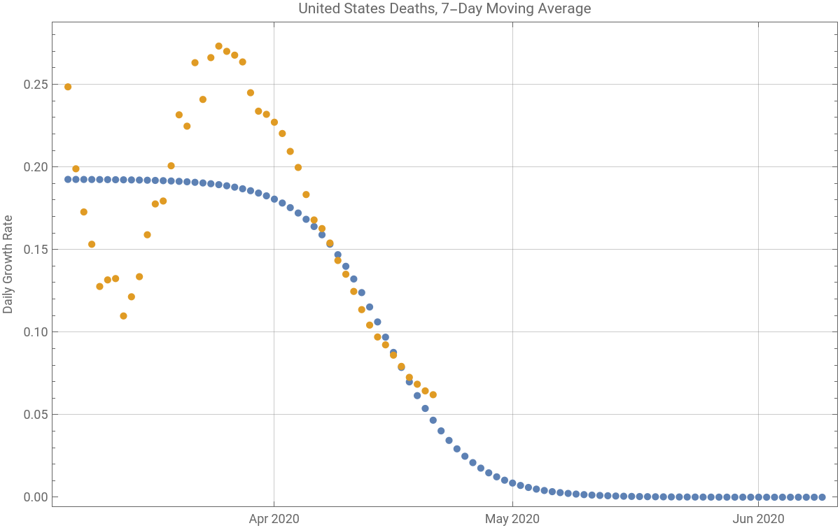
It’s interesting to note how “cleaning up” the data using a one-week moving average appears to reveal some nontrivial hidden dynamic, which does not match the behavior of the logistical function.
Also interesting to see how the logistic models evaluated as the amount of data available increases consistently underestimate both the asymptotic numbers of positives or death, and the time scale for reaching the asymptotic state. One straightforward conclusion is that the logistic function may not be a very good choice as a first-order approximation. This conclusion is also supported by the growth rate plots above.