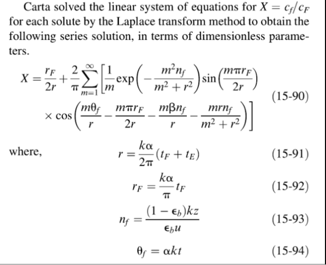
The notebook gives an implementation of Carta’s (1988) exact series solution (Eq. 15‑90 in Ref. 1) for periodic-pulse chromatography, applied to Example 15.16’s glucose/sucrose/fructose separation (see Ref. 1). Computes each solute’s dimensionless effluent concentration X(t) from its mass-transfer and equilibrium parameters, then windows the (mathematically periodic) solution around each solute’s estimated retention time to isolate the physically meaningful single-pulse peak — avoiding the spurious repeat artifacts that appear if the periodic formula is plotted over multiple cycles.
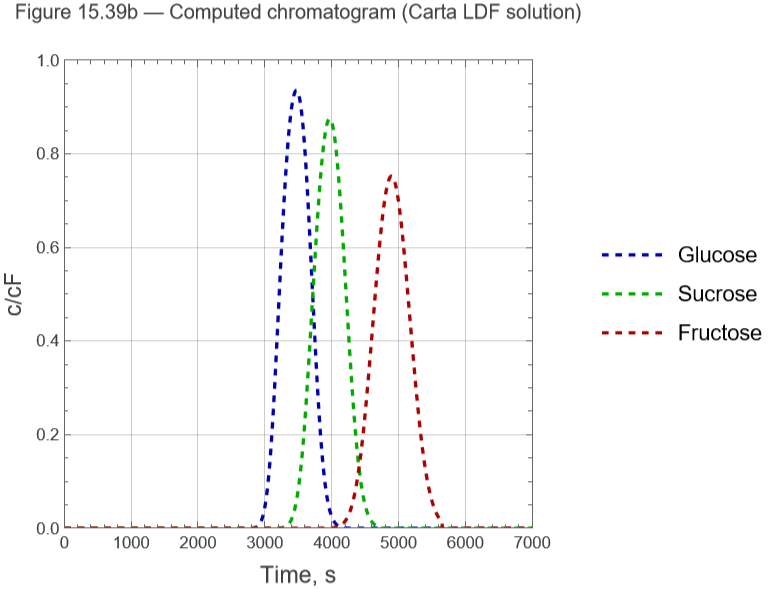
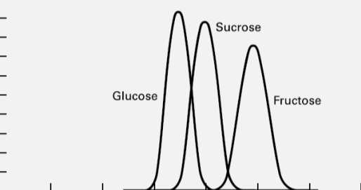
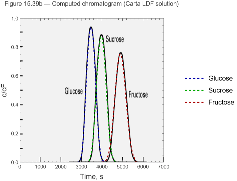
Case Study 1 reproduces the three overlapping breakthrough/elution curves of Fig. 15.39b (given in Ref. 1) for the base-case, short column (z=182 cm).
Case Studies 2–5 extend the analysis with a peak-to-peak resolution criterion, Rs = (t2-t1)/(0.5*(w1+w2)), to quantify how the separation improves as the operating conditions are changed:
● Case Study 2 increases the column length (z by a factor of 2.3);
● Case Study 3 decreases the superficial velocity (u by a factor of 2.3, i.e. longer residence time in the same column);
● Case Study 4 shortens the feed pulse duration, t_F, alone;
and
and
● Case Study 5 combines a shorter feed pulse with a longer column.
Consistent with Carta’s and Seader’s discussion, all three levers (longer column, slower flow/longer residence time, shorter feed pulse) improve resolution, with the combined case (Case Study 5) giving the sharpest, most nearly baseline-separated peaks (obtained when Rs is arounf 1.5).
and
Case Study 1 (the Base Case Study)
Case Study 1 (the Base Case Study)
Reproduction of Figure 15.39b (Ref. 1 Example 15.16)
ClearAll[X,Xwindowed,params,mMax,tauIdeal,plot];
Column’s operating conditions, Example 15.16
z is the packing length of the chromatographic column in cm
z=182;
u=0.0795;
u is the superficial (fluid) velocity of the mobile phase through the packed bed —how fast the carrier fluid moves through the column, based on the empty (unpacked) cross-sectional area. u is expressed in cm/s
u is what turns the column length z into a timescale: z/u≈2289 s is the time it takes fluid alone to traverse the 182 cm bed
u is what turns the column length z into a timescale: z/u≈2289 s is the time it takes fluid alone to traverse the 182 cm bed
Bed void fraction
epsb=0.39;
t_F and t_E are the durations of the two parts of one feed cycle in this periodic chromatographic operation:
t_F—feed (injection) pulse duration.The length of time the column is fed the solute at concentration C_F.In Example 15.16,t_F=500 s.
t_E—elution period duration.The length of time after the feed pulse ends during which pure eluent (no solute) flows through the column,washing/eluting the adsorbed solute out.In Example 15.16,t_E=2000 s.
Period = 2500 s
tF=500;tE=2000;period=tF+tE;
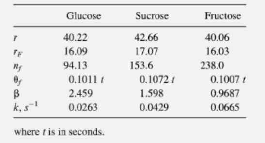
Table (p. 608): 1/alpha, r, rF, nf, beta, thetaFCoef (theta_f = thetaFCoef*t)
In[]:=
params=<|"Glucose"-><|"invAlpha"->0.26,"r"->40.22,"rF"->16.09,"nf"->94.13,"beta"->2.459,"thetaFCoef"->0.1011|>,"Sucrose"-><|"invAlpha"->0.40,"r"->42.66,"rF"->17.07,"nf"->153.6,"beta"->1.598,"thetaFCoef"->0.1072|>,"Fructose"-><|"invAlpha"->0.66,"r"->40.06,"rF"->16.03,"nf"->238.0,"beta"->0.9687,"thetaFCoef"->0.1007|>|>;
This is the number of terms in the truncated Fourier series
mMax=400;
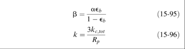
Eq.(15-90) series solution from Ref. 1-2
X[t_?NumericQ,p_Association]:=Module[{r,rF,nf,beta,thetaF},r=p["r"];rF=p["rF"];nf=p["nf"];beta=p["beta"];thetaF=p["thetaFCoef"]*t;rF/(2r)+(2/Pi)*Sum[(1/m)*Exp[-m^2*nf/(m^2+r^2)]*Sin[m*Pi*rF/(2r)]*Cos[m*thetaF/r-m*Pi*rF/(2r)-m*beta*nf/r-m*r*nf/(m^2+r^2)],{m,1,mMax}]];
Ideal (local-equilibrium) retention time estimate for each solute:
tau = (z/u) * [epsb + (1-epsb)*(1/alpha)] / epsb
tau = (z/u) * [epsb + (1-epsb)*(1/alpha)] / epsb
tauIdeal[p_Association]:=(z/u)*(epsb+(1-epsb)*p["invAlpha"])/epsb;
Window each curve to ONE period centered on its ideal retention time, so the spurious periodic repeats (at tau +/- 1*period, +/- 2*period, ...) are excluded. Half-width 0.4*period keeps a safety margin < 0.5*period.
halfWidth=0.4*period;
In[]:=
Xwindowed[t_?NumericQ,name_String]:=Module[{p=params[name],tau},tau=tauIdeal[p];If[Abs[t-tau]<=halfWidth,X[t,p],0]];
In[]:=
tMax=7000;
plot=PlotEvaluate[Table[Xwindowed[t,name],{name,{"Glucose","Sucrose","Fructose"}}]],{t,0,tMax},
Out[]=
In[]:=
IMG=
;
In[]:=
Show[plot,Prolog->{Raster[ImageData[IMG,DataReversed->True],{Scaled[{0.002,0.0}],Scaled[{1,1.0}]}]}]
Out[]=
Locate the peak by maximizing over the solute’s own valid window
Base width at a given fraction (default 5%) of the peak height found by locating the two times (left and right of the peak) where X(t) crosses frac*peakHeight.
Resolution between two adjacent (in elution order) solutes
Peak times, widths, and Rs for each adjacent pair, in elution order
Case Study 2
Case Study 2
Increase column length
Eq.(15-90) series solution from Ref. 1-2
Ideal (local-equilibrium) retention time estimate for each solute:
tau = (z/u) * [epsb + (1-epsb)*(1/alpha)] / epsb
tau = (z/u) * [epsb + (1-epsb)*(1/alpha)] / epsb
Window each curve to ONE period centered on its ideal retention time, so the spurious periodic repeats (at tau +/- 1*period, +/- 2*period, ...) are excluded. Half-width 0.4*period keeps a safety margin < 0.5*period.
Peak times, widths, and Rs for each adjacent pair, in elution order
Case Study 3
Case Study 3
Decrease superficial velocity
Eq.(15-90) series solution from Ref. 1-2
Ideal (local-equilibrium) retention time estimate for each solute:
tau = (z/u) * [epsb + (1-epsb)*(1/alpha)] / epsb
tau = (z/u) * [epsb + (1-epsb)*(1/alpha)] / epsb
Window each curve to ONE period centered on its ideal retention time, so the spurious periodic repeats (at tau +/- 1*period, +/- 2*period, ...) are excluded. Half-width 0.4*period keeps a safety margin < 0.5*period.
Peak times, widths, and Rs for each adjacent pair, in elution order
Case Study 4
Case Study 4
Shorten the feed pulse
Column’s operating conditions, Example 15.16
z is the packing length of the chromatographic column in cm
u is the superficial (fluid) velocity of the mobile phase through the packed bed —how fast the carrier fluid moves through the column, based on the empty (unpacked) cross-sectional area. u is expressed in cm/s
u is what turns the column length z into a timescale: z/u≈2289 s is the time it takes fluid alone to traverse the 182 cm bed
u is what turns the column length z into a timescale: z/u≈2289 s is the time it takes fluid alone to traverse the 182 cm bed
Bed void fraction
t_F and t_E are the durations of the two parts of one feed cycle in this periodic chromatographic operation:
t_F—feed (injection) pulse duration.The length of time the column is fed the solute at concentration C_F.In Example 15.16,t_F=500 s.
t_E—elution period duration.The length of time after the feed pulse ends during which pure eluent (no solute) flows through the column,washing/eluting the adsorbed solute out.In Example 15.16,t_E=2000 s.
t_F—feed (injection) pulse duration.The length of time the column is fed the solute at concentration C_F.In Example 15.16,t_F=500 s.
t_E—elution period duration.The length of time after the feed pulse ends during which pure eluent (no solute) flows through the column,washing/eluting the adsorbed solute out.In Example 15.16,t_E=2000 s.
Period = 2500 s
This is the number of terms in the truncated Fourier series
Eq.(15-90) series solution from Ref. 1-2
Ideal (local-equilibrium) retention time estimate for each solute:
tau = (z/u) * [epsb + (1-epsb)*(1/alpha)] / epsb
tau = (z/u) * [epsb + (1-epsb)*(1/alpha)] / epsb
Window each curve to ONE period centered on its ideal retention time, so the spurious periodic repeats (at tau +/- 1*period, +/- 2*period, ...) are excluded. Half-width 0.4*period keeps a safety margin < 0.5*period.
Peak times, widths, and Rs for each adjacent pair, in elution order
Case Study 5
Case Study 5
Shorten the feed pulse and increase column length
Column's operating conditions, Example 15.16
z is the packing length of the chromatographic column in cm
u is the superficial (fluid) velocity of the mobile phase through the packed bed —how fast the carrier fluid moves through the column, based on the empty (unpacked) cross-sectional area. u is expressed in cm/s
u is what turns the column length z into a timescale: z/u≈2289 s is the time it takes fluid alone to traverse the 182 cm bed
u is what turns the column length z into a timescale: z/u≈2289 s is the time it takes fluid alone to traverse the 182 cm bed
Bed void fraction
t_F and t_E are the durations of the two parts of one feed cycle in this periodic chromatographic operation:
t_F—feed (injection) pulse duration.The length of time the column is fed the solute at concentration C_F.In Example 15.16,t_F=500 s.
t_E—elution period duration.The length of time after the feed pulse ends during which pure eluent (no solute) flows through the column,washing/eluting the adsorbed solute out.In Example 15.16,t_E=2000 s.
t_F—feed (injection) pulse duration.The length of time the column is fed the solute at concentration C_F.In Example 15.16,t_F=500 s.
t_E—elution period duration.The length of time after the feed pulse ends during which pure eluent (no solute) flows through the column,washing/eluting the adsorbed solute out.In Example 15.16,t_E=2000 s.
Period = 2500 s
This is the number of terms in the truncated Fourier series
Eq.(15-90) series solution from Ref. 1-2
Ideal (local-equilibrium) retention time estimate for each solute:
tau = (z/u) * [epsb + (1-epsb)*(1/alpha)] / epsb
tau = (z/u) * [epsb + (1-epsb)*(1/alpha)] / epsb
Window each curve to ONE period centered on its ideal retention time, so the spurious periodic repeats (at tau +/- 1*period, +/- 2*period, ...) are excluded. Half-width 0.4*period keeps a safety margin < 0.5*period. halfWidth = 0.4*period;
Base width at a given fraction (default 5%) of the peak height, found by locating the two times (left and right of the peak) where X(t) crosses frac*peakHeight.
Peak times, widths, and Rs for each adjacent pair, in elution order
References
References
[1] Seader, J. D., Henley, E. J., & Roper, D. K. (2011). Separation Process Principles: Chemical and Biochemical Operations (3rd ed.). Hoboken, NJ: John Wiley & Sons.
[2] Carta, G. (1988). Exact analytic solution of a mathematical model for chromatographic operations. Chemical Engineering Science, 43(10), 2877–2883. https://doi.org/10.1016/0009-2509(88)80030-7
CITE THIS NOTEBOOK
CITE THIS NOTEBOOK
Carta's analytic chromatogram for glucose-sucrose-fructose separation
by Housam Binous
Wolfram Community, STAFF PICKS, August 10, 2026
https://community.wolfram.com/groups/-/m/t/3776120
by Housam Binous
Wolfram Community, STAFF PICKS, August 10, 2026
https://community.wolfram.com/groups/-/m/t/3776120