In many chemistry classrooms, Lewis structures are commonly used to predict electron-pair geometry, bond angles, and shape. While these diagrams are useful, they end up providing misleading information on the intramolecular interactions. In this essay, the focus is shifted to constructing molecular orbital diagrams, following along molecular orbital theory. We explore how much more comprehensive and accurate MO diagrams are. With computational optimization techniques like Hartree-Fock, orbital interactions can be more clearly visualized. We determine electron configurations, determining which are filled, vacant, or are occupied by a single electron.
Introduction
Introduction
Understanding atomic bonding has been a central quest in chemistry. While Lewis structures offer useful predictions about geometry, they often fall short in explaining certain phenomena. An example is paramagnetism in . According to the Lewis structure, there are no unpaired electrons. However, it displays the strange behavior of being attracted to magnetic fields though it is clearly not magnetic by itself. How do we account for these changes and experimental differences, especially in a simple diatomic molecule such as ?
O
2
H
2
This is where molecular orbital theory comes into play. Molecular orbital theory provides a visual for the distribution of electrons in molecules, as it gives the regions of space electrons will likely be found. It offers more comprehensive explanations for bonding in other molecules, like those that violate the octet rules or follow other complicated patterns. Visualizing molecular orbitals is essential to understanding how atoms truly interact. Seeing and understanding the diagrams explains how processes like delocalization occur, and paint a more accurate picture that clear the misconceptions about bonding. Molecular orbitals (MOs) also allow us to predict how stable a bonding will be. The existence of both bonding and antibonding orbitals display two compounds will interact, and specifically how the electrons will behave.Figure 1. A sample MO diagram of a homonuclear diatomic molecule. From Reference 1
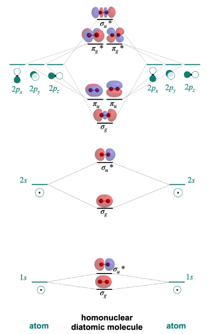
Lewis structures are commonly used to predict electron-pair geometry, bond angles, and molecular geometry. While Lewis structures provide accurate results, there are several issues and inaccurate information. Using molecular orbitals, the combination of atomic orbitals, offers more comprehensive explanations for bonding in other molecules, such as those that violate the octet rules or follow other complicated patterns. Each atom has its own atomic orbitals, which then overlap in complex ways to give molecular orbitals. A mathematical process called LCAO provides approximations on the orbitals. LCAO, or linear combination of atomic orbitals, uses the wave like properties of electrons for our predictions. Molecular orbitals are the combinations of the individual atomic orbital wave functions, which combine in two ways.
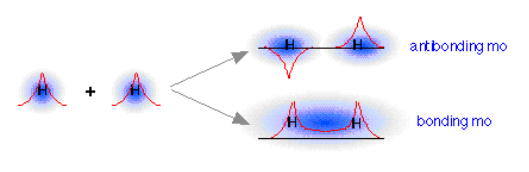
When atomic orbitals combine , the wave like properties of an electron become relevant since molecular orbitals are the combinations of individual atomic orbital wave functions. There are two ways waves combine: constructive interference and destructive interference. The in-phase addition in constructive interference produces a lower energy σ molecular orbital where most of the electron density is directly between the nuclei of the atoms, which we then call a bonding orbital. The out-of-phase addition, destructive interference, produces a higher energy sigma-s-star molecular orbital where there is a node. Because of the high energy, an electron will be not be found in these areas and they form antibonding orbitals.Figure 2. A display of how the waves of two hydrogen atoms combine in two ways. The constructive interference makes the bonding MO, while the destructive interference creates the antibonding MO. From Reference 2
Finding Optimal Electron Structure with HartreeFock
Finding Optimal Electron Structure with HartreeFock
First, the molecular orbitals must be optimized prior to visualizing them. To compute that optimal orbital, one can utilize the Hartree-Fock approach, which approximates the wave function through an iterative process. Each time, the approximate get closer to the optimal orbital and minimize the total electronic energy, which is important to create the most stable system. Once we have these structures, it is clear that they describe delocalized electrons a lot better than Lewis structures where electrons are assigned to certain elements. Accurate visualization has uses in drug design, materials science, and photochemistry and electron distributions explain reactivity, absorption properties, or catalytic activity.To spit out the most accurate molecular orbital visual, we begin with optimizing the compound. Say we begin with , consisting of two hydrogen molecules with a single bond. We use HartreeFock to set a default method to construct this. Our basis set is STO-3G, which gives us a version of the molecule’s wavefunction. Each function is build from three Gaussian functions it gives us a less accurate representation of the actual orbital, the Slater-Type Orbital (STO) which closely resembles real atomic orbitals.
H
2
Load the quantum chemistry paclet.
In[]:=
Needs["WolframChemistry`QuantumChemistry`"]
Set our default optimization method to HartreeFock with a basis set of STO-3G:
In[]:=
default=ModelChemistry["HartreeFock","STO-3G"]
Out[]=
ModelChemistry[HartreeFock,STO-3G]
Define our molecule hydrogen and optimize it utilizing HartreeFock, assigning it as our “optimal”:
In[]:=
hydrogen=Molecule["Hydrogen"]optH=CloudGet[CloudObject[
https://www.wolframcloud.com/obj/adicov20/optH
]];Out[]=
Molecule


The structure here is the one with the bond length that minimizes energy. This minimum energy is calculated with a fundamental equation in quantum chemistry, the time-independent Schrödinger equation which says the following:
The structure here is the one with the bond length that minimizes energy. This minimum energy is calculated with a fundamental equation in quantum chemistry, the time-independent Schrödinger equation which says the following:
In[]:=
HoldForm[H*Ψ="E"*Ψ]
Out[]=
HΨ=EΨ
We approximate the wave function, Ψ, which tells us everything about electrons such as their location, behavior, and more. The equation tells us that with the wave function, we have a certain energy . While we cannot exactly solve Schrödinger’s equation, we can use a basis set to build or approximate the wave function. Here we played with the parameters and approximated the lowest E we can get, which we can see.
E
Fetch the energy of the optimized configuration:
In[]:=
Out[]=
The MO diagram of hydrogen is a simple example with only two molecular orbitals, as each hydrogen has one 1s atomic orbital. One of them is the LUMO (lowest unoccupied molecular orbital) and the other is the HOMO (highest occupied molecular orbital). In our MO diagram, we want to include everything below the HOMO because those are filled orbitals.
Visual of HOMO for our optimized hydrogen structure:
In[]:=
Out[]=

What we see is one circular orbital, where the two orbitals overlapped and together created a bonding orbital. Since we had two atomic orbitals, one from each hydrogen, we must have two total.
Visual of LUMO for our optimized hydrogen structure:
In[]:=
Out[]=

The other is an antibonding orbital where we see a gap in the middle. This gap is the node, where energy level is so high, electrons are not found there. The purpose of the MO diagram is to display all of these orbitals, both bonding and antibonding. We can also accurately place these orbitals based on energy to get a more accurate picture.
Systemizing the distribution of electrons in orbitals with Aufbau Principle, Pauli Exclusion Principle, and the Hund’s rule
Systemizing the distribution of electrons in orbitals with Aufbau Principle, Pauli Exclusion Principle, and the Hund’s rule
Each orbital can hold up to two electrons, and the way orbitals fill up has a couple rules and principles.
Making functions to display graphics for half, full, and empty orbitals.
In[]:=
electronArrow[x_,y_]:=Graphics[{Thickness[0.05],Line[{{x,y},{x,y+2},{x-0.5,y+1}}]}]half[x_,y_]:=Graphics[{Sequence@@electronArrow[x,y],Thickness[0.05],Line[{{x-0.5,y-0.2},{x+1,y-0.2}}]},ImageSize->40]full[x_,y_]:=Graphics[{Sequence@@electronArrow[x,y],Thickness[0.05],Line[{{x-0.5,y-0.2},{x+1,y-0.2}}],Rotate[Sequence@@electronArrow[x+1,y],Pi]},ImageSize->40]empty[x_,y_]:=Graphics[{Thickness[0.05],Line[{{x-0.5,y-0.2},{x+1,y-0.2}}]},ImageSize->40]
The first is Aufbau Principle, which states that electrons fill the lowest energy molecular orbitals first. That means electrons will first fill 1s, then 2s, 2p, 3s and onwards. Previously, we touched on how orbitals can only hold up to two electrons. It is according to Pauli Exclusion Principle that these electrons have opposite spins, ensuring no two electrons have the same set of quantum numbers. Finally, there is Hund’s Rule, which says that with multiple degenerate orbitals that have the same energy, electrons fill them one at a time first. This way of filling ensures the electrons occupy as many orbitals are possible and results in more electrons with parallel spins; more electrons with the same spin maximizes total spin and stabilizes the molecule.
According to the rules and principles, filling a p orbital with 3 electrons would look like this:
Filling a d orbital with 7 electrons would look like this:
Defining a function that fills an array with 1 electron each, then goes through and fills more if they exist. The code matches the label of the orbital to its occupancy.
Now that we have the function that fills orbitals given the number of electrons, we need to pass in the number of electrons so it can conclude the orbitals they will fill up. We also desire to get the energies of each orbital. This way, the orbitals can be mapped to their corresponding energy and placed accurately and accordingly in the final graphic .
Finding the optimal molecular geometry structure for the input molecule:
Total the number of electrons (atomic number) for each atom in the compound:
Retrieve energies of each molecular orbital in the compound:
The orbitals must fill in increasing level of energy according to Aufbau. We must also keep in mind each type orbital has different numbers of electrons it can hold. For example, s subshells only have 1 orbital and can therefore only hold 2 electrons. Keeping track of which orbital can hold what, and when the electrons must occupy the next lowest orbital is necessary.
Create array of orbitals and occupancy and apply the orbitalFilling function.
Assembling the visual components
Assembling the visual components
Ensure our amount of orbital labels equals the amount of orbital energies in order to pair them together. Draw the various lines and connections found in MO diagrams.
Finally, we join all the elements together into one graphic.
Creating the final function
Creating the final function
Finally, the function has to accept input. Wolfram supports several different kinds of input for molecules such as Entity and Molecule. The function could also accept a string, as long as it is recognizable as a Molecule. We must ensure that if we do not have a recognizable input, the function stops running. Additionally, since the function is focusing solely on diatomic molecules, it’s important to test for the AtomCount. After testing for the right conditions, we call for drawMODiagram to get our final graphic, the MO diagram for whichever molecule we had put in.
Define different functions to check for several types of input and ensure it matches what the function can handle.
Conclusion
Conclusion
The wave-like properties of electrons means that their role in bonding is a lot more than just a shared dot or line in a 2D structure. Electrons instead exist in regions, in orbitals with unique shapes based on its set of quantum numbers. With the wave function from quantum mechanics, one acquires much more information on the crazy states of these particles. Molecular orbitals are where electron clouds overlap, forming entirely new clouds of probability, influencing stability, reactivity, and shape overall. Molecular orbitals offer an entirely new perspective into the geometry of chemistry, beyond what simpler diagrams such as Lewis structures display. MO diagrams reveal how atoms unite in molecules through the properties of electron distribution and quantum mechanics. Understanding these processes and molecular orbital theory, we gain insight into bonding and anti-bonding interactions, the stability of molecules, several intramolecular properties. The knowledge we can draw from this extends beyond chemistry and into other areas where we don’t realize how much chemistry there is, like computational fields and materials science.
Future Directions
Future Directions
Accurately determining atomic energies and generating precise representations will require diverse software and advanced computational functions. Currently, my focus is on optimizing processes for simpler systems, but I envision it extending to handle polyatomic compounds in the future. Heteronuclear molecules and larger polyatomic species will intensify the challenge due to additional factors like molecular symmetry, electronic interactions, and other geometric intricacies. Both deeper theoretical research and specialized software will help with insightful chemical modelling and further enhancing our understanding of molecular behavior on a fundamental level. With a higher accuracy comes an increased scope of use. With MO diagrams, one can simulate spectroscopic properties and link MO energies with other observable properties. One could also generate and analyze visual electron cloud distributions from the MO information.
After refining the function to be able to evaluate these properties of higher complexity, I aim to contribute the MO function as a WFR to be of use to others who wish to visualize orbitals.
After refining the function to be able to evaluate these properties of higher complexity, I aim to contribute the MO function as a WFR to be of use to others who wish to visualize orbitals.
Acknowledgements
Acknowledgements
I would like to thank Jason Sonnenberg, my mentor, for his invaluable guidance and support throughout the project. Without his ideas and vision, this would not have been possible. I also thank Jason Biggs for allowing us to use his Quantum Chemistry paclet, which was fundamental to me building and working on this function. I would love to personally thank the TAs that were there when my code was broken, Bertie Bennett, Averyl Xu, and Gloria Chan, and the other wonderful TAs who were always helpful. Last but not least, I thank Eryn Gillam, Rory Foulger, and Megan Davis, our camp directors, for their constant effort and support to make this program possible.
References
References
◼
Haas, K. (2020, August 23). 4.2.1: Molecular Orbitals. Chemistry LibreTexts. https://chem.libretexts.org/Courses/Saint_Marys_College_Notre_Dame_IN/CHEM_431%3A_Inorganic_Chemistry_(Haas)/CHEM_431_Readings/04%3A_Molecular_Orbitals/4.02%3A_Homonuclear_Diatomic_Molecules/4.2.01%3A_Molecular_Orbitals
◼
Lower, S. (2022, November 13). 9.8: Molecular Orbital Theory. Chemistry LibreTexts. https://chem.libretexts.org/Bookshelves/General_Chemistry/Chem1_(Lower)/09%3A_Chemical_Bonding_and_Molecular_Structure/9.08%3A_Molecular_Orbital_Theory
◼
Molecular Orbital Theory. FSU Chemistry. (n.d.). https://www.chem.fsu.edu/chemlab/chm1046course/motheory.html
CITE THIS NOTEBOOK
CITE THIS NOTEBOOK
Visualizing diatomic molecular orbitals
by Advika Asthana
Wolfram Community, STAFF PICKS, July 11, 2025
https://community.wolfram.com/groups/-/m/t/3503009
by Advika Asthana
Wolfram Community, STAFF PICKS, July 11, 2025
https://community.wolfram.com/groups/-/m/t/3503009