Contributions by: Jordan Hasler, Jeremy Stratton-Smith, Douglas Adam Smith
In[]:=
EpidemicModel[]
Out[]=


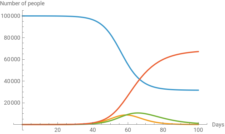


Epidemiology Introduction
Epidemiology Introduction
Throughout history, pandemics have had devastating effects. The bubonic plague led to the death of up to 1/3 of the European population between 1346 and 1350. The epidemic occurred regularly in the following 300 years. Other infectious diseases such as measles can occur regularly every year and are said to be endemic when they do. In 1918, an outbreak of influenza led to 50 million deaths. Every year influenza epidemics lead to up to 35000 deaths in the United States. (1)
In 2018, 1.5 million people died from tuberculosis with up to 10 million people becoming infected. Multidrug-resistant TB is estimated have happened in 484,000 cases. Between 2000 and 2018, diagnosis and treatment is believed to have saved 58 million lives. Up to one quarter of the world’s population has latent TB meaning that they are not yet ill from the disease and are not able to spread it. In 2017, there were over 219 million cases of malaria with as many as 435000 deaths. (2, 3)
The novel Coronavirus (COVID-19) has led to a pandemic in early 2020. As of April 2nd, with over 931,578 cases and 46,792 deaths. (16)
The modern viewpoint of infectious disease is that illness is spread by viruses and bacteria through person-to-person contact between infectious and susceptible individuals. In 1906, W.H. Hamer created a model of infectious disease spread that maintained disease spread happens at a rate proportional to both the number of susceptible and number of infected individuals. (4) Pioneered in the 1927 paper of Kermack and McKendrick, compartmental based models divide the population into groups, called compartments, and aim to describe the flow of people among these compartments over time as the disease spreads. (5) Compartments may include the number of susceptible, infected, and recovered individuals. Specific compartment based models differ in the particular compartments included and in the ways in which such compartments are related to one another
In order to accurately model the movement of people between these compartments, we need to consider at what rates they do so. In this case, a rate of a change is modeled using a differential equation which relates a set of functions with their derivatives. In some cases, we are able to find explicit functions to solve the differential equations, while in other cases we resort to using numerical methods when no analytical solution exists. For instance, Thomas Malthus when studying the growth of a population, assumed that population growth was proportional to the current population size: which leads to the solution . (9)
The aim of this post is to highlight a few compartmental models and illuminate the disease progression as well as the motivation for developing different models.
For each model described, we include a graphical representation of the model, a description of any new parameters and/or compartments, the differential equations for the model and an interactive representation of the model that was developed by members of the Wolfram|Alpha Math Team. EpidemicModel[] will soon be available through the Wolfram Function Repository, but the code is also included at the end of this post.
In 2018, 1.5 million people died from tuberculosis with up to 10 million people becoming infected. Multidrug-resistant TB is estimated have happened in 484,000 cases. Between 2000 and 2018, diagnosis and treatment is believed to have saved 58 million lives. Up to one quarter of the world’s population has latent TB meaning that they are not yet ill from the disease and are not able to spread it. In 2017, there were over 219 million cases of malaria with as many as 435000 deaths. (2, 3)
The novel Coronavirus (COVID-19) has led to a pandemic in early 2020. As of April 2nd, with over 931,578 cases and 46,792 deaths. (16)
The modern viewpoint of infectious disease is that illness is spread by viruses and bacteria through person-to-person contact between infectious and susceptible individuals. In 1906, W.H. Hamer created a model of infectious disease spread that maintained disease spread happens at a rate proportional to both the number of susceptible and number of infected individuals. (4) Pioneered in the 1927 paper of Kermack and McKendrick, compartmental based models divide the population into groups, called compartments, and aim to describe the flow of people among these compartments over time as the disease spreads. (5) Compartments may include the number of susceptible, infected, and recovered individuals. Specific compartment based models differ in the particular compartments included and in the ways in which such compartments are related to one another
In order to accurately model the movement of people between these compartments, we need to consider at what rates they do so. In this case, a rate of a change is modeled using a differential equation which relates a set of functions with their derivatives. In some cases, we are able to find explicit functions to solve the differential equations, while in other cases we resort to using numerical methods when no analytical solution exists. For instance, Thomas Malthus when studying the growth of a population, assumed that population growth was proportional to the current population size:
p'[t]kp
p(t)=a
kt
e
The aim of this post is to highlight a few compartmental models and illuminate the disease progression as well as the motivation for developing different models.
For each model described, we include a graphical representation of the model, a description of any new parameters and/or compartments, the differential equations for the model and an interactive representation of the model that was developed by members of the Wolfram|Alpha Math Team. EpidemicModel[] will soon be available through the Wolfram Function Repository, but the code is also included at the end of this post.
SI Model
SI Model
Out[]=

Let’s take a look at a relatively large population of 100,001 individuals (roughly the size of a small city), one of which is infected. We break the population into two compartments: Susceptible (S) and Infected (I). We will assume that the population size is fixed. We can further suppose that there is no travel. Furthermore, we assume that the population is homogeneously connected. This means that an infection event could happen between any of the susceptible-infected pairs–the system is all-to-all. In other words, all individuals are equally likely to coming into contact with one another. Note that since only contacts with a susceptible person can lead to new infections, we assume that the change in susceptible population will depend upon the proportion of susceptible individuals in the population .Therefore, we assume that . Since we assumed the population size was fixed at individuals, we know that . By taking the derivative of both sides, we see that , or that . Hence, . Finally, we need to determine the proportionality constant for and . β will represent the transmission rate and is the proportionality constant for . Since the number of susceptible individuals will decrease over time, will be negative, while will be positive. This leads us to the differential equations: and .
S[t]
n
S'[t]∝I[t]
S[t]
n
n
S[t]+I[t]=n
S'[t]+I'[t]=0
S'[t]=-I'[t]
I'[t]∝
S[t]
n
I[t]
S'[t]
I'[t]
S'[t]
S'[t]
I'[t]
S'[t]=-βI[t]
S[t]
n
I'[t]=βI[t]
S[t]
n
Note that in the equations and code we use in place of due to capital I representing the imaginary number in the Wolfram Language.
Inf
I
Sqrt[-1]
Out[]=
Equations |
′ S βInf[t]S[t] n |
′ Inf βInf[t]S[t] n |
S[0]s0 |
Inf[0]i0 |
Inf[t]+S[t]n |

Variables | |
t | time measured in days |
S[t] | number of susceptible at time t |
Inf[t] | number of infected at time t |
β | infection rate |
n | total population (s0 + i0) |
The model
The model
In[]:=
EpidemicModel["SI"]
Out[]=
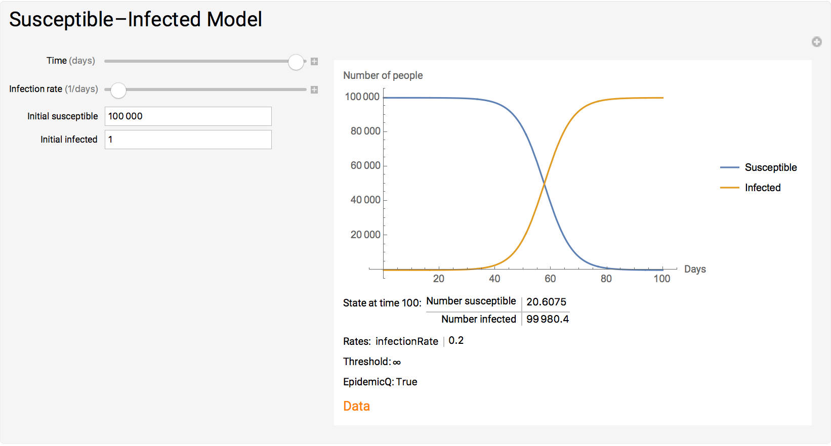
We can see that as the infection rate increases, everyone becomes infected sooner, but in this model everyone does eventually become infected. As such, in the SI model we always have an epidemic.
Solving the equations
Solving the equations
SIS Model
SIS Model
Out[]=
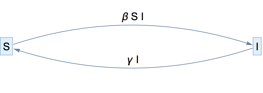
The Susceptible–Infected–Susceptible (SIS) model builds on the SI model by adding in the possibility that those who become infected can recover and return to the compartment. In this way, the SIS model does not introduce any new compartments, but introduces the possibility of recovery. The rate of recovery is represented in the model graph by the parameter . Introducing recovery changes the differential equations for this model by not only taking away from but by also taking away from I at the rate of .
S
γ
S
γ*I
Out[]=
Equations |
′ S βInf[t]S[t] n |
′ Inf βInf[t]S[t] n |
S[0]s0 |
Inf[0]i0 |
Inf[t]+S[t]n |
Variables | |
t | time measured in days |
S[t] | number of susceptible at time t |
Inf[t] | number of infected at time t |
β | infection rate |
γ | rate of recovery |
n | total population (i0 + s0) |
The model
The model
EpidemicModel["SIS"]
Out[]=
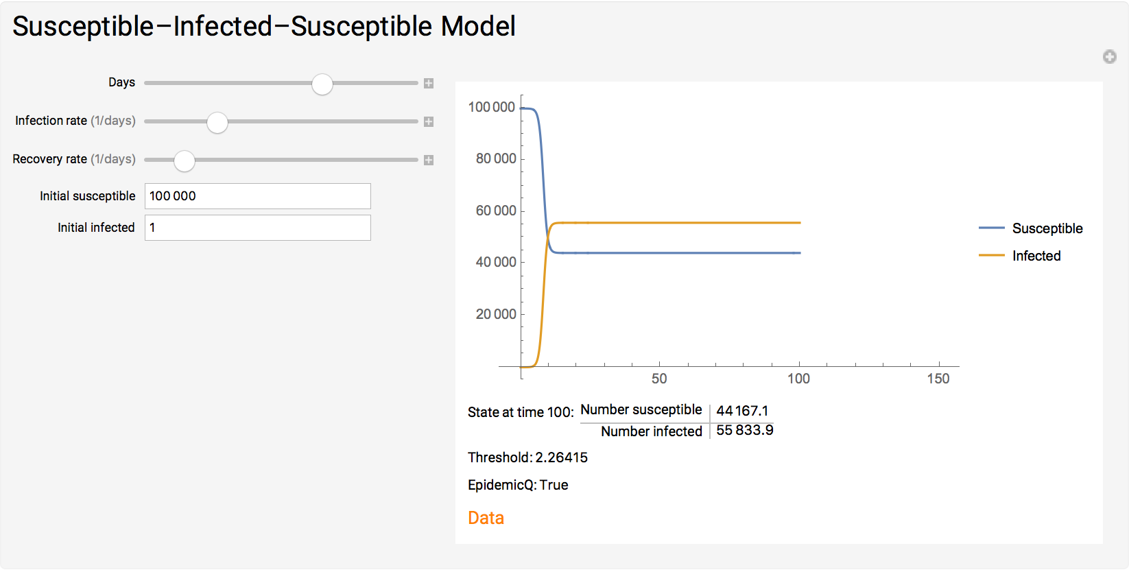
As seen in the above example, the possibility of recovery means that, rather than everyone eventually becoming infected as in the SI model, the system can reach an equilibrium state. This equilibrium happens when the same number of people are becoming infected as are recovering so that there is a balance between the and compartments. Changing the infection rate and recovery rate influences both how quickly this equilibrium is reached and what the ultimate equilibrium state is, provided the infection rate is greater than the recovery rate.
S
I
Additionally, unlike the SI model, in the SIS model, the value labeled “Threshold” changes as the infection and recovery rates change. This threshold is calculated in different ways for each model, but is a measure of whether or not the infection takes off and becomes an epidemic. In this case, we have calculated the threshold assuming an initial state of one infected individual.
Finding the steady state
Finding the steady state
SIR Model
SIR Model
Out[]=

The Susceptible-Infected-Recovered model, in contrast to the SI model, accounts for the possibility of recovery by adding another compartment, Recovered (R).
Note that we can rewrite the infected compartment as:
An epidemic will occur when:
for an epidemic to occur.
The model
The model
Note that when the recovery rate is greater than the infection rate, the threshold is greater than 1 and we have an epidemic.
SEIR Model
SEIR Model
The model
The model
As the transmission rate increases, the exposed population more quickly moves on to become infected, as is indicated by the flattening of the Exposed curve in the interactive model. Additionally, for the same infection and recovery rates, our SEIR model will have the same threshold value, but a potential epidemic will be slowed down due to the delay in individuals becoming infected.
SVIR Model
SVIR Model
The model
The model
SIQR Model
SIQR Model
The model
The model
SPIR Model
SPIR Model
The model
The model
In the SPIR model, when a person is infected, there is a chance that they go into the power-spreader compartment. If they do so, they will spread the infection at an increased rate for the duration of their contagious period. Playing with the settings in the visualization above, you will see that power infector probability and recovery rate dramatically affect the result of the outbreak.
Some epidemics are known for the involvement of power spreaders and power spreading events. The 2002 SARS epidemic is one example of this, in which models involving a power spreader compartment were more appropriate than others. Some models account for power spreader events, but it should be noted that the above visualization focuses on power spreader individuals.
Some epidemics are known for the involvement of power spreaders and power spreading events. The 2002 SARS epidemic is one example of this, in which models involving a power spreader compartment were more appropriate than others. Some models account for power spreader events, but it should be noted that the above visualization focuses on power spreader individuals.
Extensions
Extensions
We made many different assumptions while formulating the system of equations for each different model. Our models assume that each person in the population is equally likely to come into contact with everyone else. There are several ways to model epidemics that do not make this assumption. One way is modeling the potentially-heterogeneous networks of contact between people, and another way is by using stochastic models. In reality, networks of contact among individuals are usually heterogeneous, and as such, we need models that take this into account. Such models add complexity to represent social and geographic factors that divide up populations. (15) Rather than focusing on the continuous flow between compartments, stochastic models take into account the transition probabilities of particular events.
Conclusion
Conclusion
These compartment-based models are useful for making predictions about the spread of infectious disease, but ultimately a model is only as good as the assumptions that it is built upon. After building a model, the next task is to use real world data to determine if it is an appropriate model for the given situation, and if so, to fine tune the parameters of the model and make predictions about how the disease might spread.
References
References
(1) Brauer, Fred. “Mathematical Epidemiology: Past, Present, and Future.” Infectious Disease Modelling, vol. 2, no. 2, May 2017, pp. 113–27. ScienceDirect, doi:10.1016/j.idm.2017.02.001.
(2) Tuberculosis (TB). https://www.who.int/news-room/fact-sheets/detail/tuberculosis.
(3) Malaria. https://www.who.int/data/gho/data/themes/malaria/GHO/malaria
(4) Brauer, Fred, et al. Mathematical Models in Epidemiology. Springer New York, 2008
(5) Dietz, K. “The Estimation of the Basic Reproduction Number for Infectious Diseases.” Statistical Methods in Medical Research, vol. 2, no. 1, Mar. 1993, pp. 23–41. SAGE Journals.
(6) Herrerías-Azcué, Francisco, et al. “Stirring Does Not Make Populations Well Mixed.” Scientific Reports, vol. 8, Mar. 2018. PubMed Central.
(7) Small, Michael. Dynamics of Biological Systems. CRC Press, 2012.
(8) Kiss, István Z., et al. Mathematics of Epidemics on Networks: From Exact to Approximate Models. Springer International Publishing, 2017.
(9) Zill, Dennis G. A First Course in Differential Equations with Modeling Applications. 9th ed, Brooks/Cole, Cengage Learning, 2009.
(10) Vestergaard, Christian L., and Mathieu Génois. “Temporal Gillespie Algorithm: Fast Simulation of Contagion Processes on Time-Varying Networks.” PLOS Computational Biology, vol. 11, no. 10, Oct. 2015, p. e1004579. PLoS Journals.
(11) Balcan, Duygu, et al. Multiscale mobility networks and the spatial spreading of infectious diseases. PNAS. vol. 106, no. 51, Dec. 2009.
(12) Pastor-Satorras, Romualdo, and Alessandro Vespignani. “Epidemic Spreading in Scale-Free Networks.” Physical Review Letters, vol. 86, no. 14, Apr. 2001, pp. 3200–03. APS.
(13) Escalante, René, and Marco Odehnal. “A Deterministic Mathematical Model for the Spread of Two Rumors.” ArXiv:1709.01726 [Physics], 1, Sept. 2017.
(14) Woo, Jiyoung, and Hsinchun Chen. “Epidemic Model for Information Diffusion in Web Forums: Experiments in Marketing Exchange and Political Dialog.” SpringerPlus, vol. 5, Jan. 2016. PubMed Central.
(15) Volz, Erik, and Lauren Ancel Meyers. “Susceptible–Infected–Recovered Epidemics in Dynamic Contact Networks.” Proceedings of the Royal Society B: Biological Sciences, vol. 274, no. 1628, Dec. 2007, pp. 2925–33. PubMed Central.
(16) https://www.wolframcloud.com/obj/examples/COVID19World
(17) Mkhatshwa, Thembinkosi, and Anna Mummert. “Modeling Super-Spreading Events for Infectious Diseases: Case Study SARS.” ArXiv:1007.0908 [q-Bio], Oct. 2010.
(18) Severe Acute Respiratory Syndrome --- Singapore, 2003. https://www.cdc.gov/mmwr/preview/mmwrhtml/mm5218a1.htm.
(2) Tuberculosis (TB). https://www.who.int/news-room/fact-sheets/detail/tuberculosis.
(3) Malaria. https://www.who.int/data/gho/data/themes/malaria/GHO/malaria
(4) Brauer, Fred, et al. Mathematical Models in Epidemiology. Springer New York, 2008
(5) Dietz, K. “The Estimation of the Basic Reproduction Number for Infectious Diseases.” Statistical Methods in Medical Research, vol. 2, no. 1, Mar. 1993, pp. 23–41. SAGE Journals.
(6) Herrerías-Azcué, Francisco, et al. “Stirring Does Not Make Populations Well Mixed.” Scientific Reports, vol. 8, Mar. 2018. PubMed Central.
(7) Small, Michael. Dynamics of Biological Systems. CRC Press, 2012.
(8) Kiss, István Z., et al. Mathematics of Epidemics on Networks: From Exact to Approximate Models. Springer International Publishing, 2017.
(9) Zill, Dennis G. A First Course in Differential Equations with Modeling Applications. 9th ed, Brooks/Cole, Cengage Learning, 2009.
(10) Vestergaard, Christian L., and Mathieu Génois. “Temporal Gillespie Algorithm: Fast Simulation of Contagion Processes on Time-Varying Networks.” PLOS Computational Biology, vol. 11, no. 10, Oct. 2015, p. e1004579. PLoS Journals.
(11) Balcan, Duygu, et al. Multiscale mobility networks and the spatial spreading of infectious diseases. PNAS. vol. 106, no. 51, Dec. 2009.
(12) Pastor-Satorras, Romualdo, and Alessandro Vespignani. “Epidemic Spreading in Scale-Free Networks.” Physical Review Letters, vol. 86, no. 14, Apr. 2001, pp. 3200–03. APS.
(13) Escalante, René, and Marco Odehnal. “A Deterministic Mathematical Model for the Spread of Two Rumors.” ArXiv:1709.01726 [Physics], 1, Sept. 2017.
(14) Woo, Jiyoung, and Hsinchun Chen. “Epidemic Model for Information Diffusion in Web Forums: Experiments in Marketing Exchange and Political Dialog.” SpringerPlus, vol. 5, Jan. 2016. PubMed Central.
(15) Volz, Erik, and Lauren Ancel Meyers. “Susceptible–Infected–Recovered Epidemics in Dynamic Contact Networks.” Proceedings of the Royal Society B: Biological Sciences, vol. 274, no. 1628, Dec. 2007, pp. 2925–33. PubMed Central.
(16) https://www.wolframcloud.com/obj/examples/COVID19World
(17) Mkhatshwa, Thembinkosi, and Anna Mummert. “Modeling Super-Spreading Events for Infectious Diseases: Case Study SARS.” ArXiv:1007.0908 [q-Bio], Oct. 2010.
(18) Severe Acute Respiratory Syndrome --- Singapore, 2003. https://www.cdc.gov/mmwr/preview/mmwrhtml/mm5218a1.htm.