Power Spectrum of Sinusoidal Signals
Authors: Housam Binous and Ahmed Bellagi
Power Spectrum of Sinusoidal Signals
Authors: Housam Binous and Ahmed Bellagi
Authors: Housam Binous and Ahmed Bellagi
We compute the power spectra of sinusoidal signals with and without noise. Such spectra display the distribution of power contained within the signal over frequency.
This signal representation is often simpler to analyze than its time-domain counterpart.
This signal representation is often simpler to analyze than its time-domain counterpart.
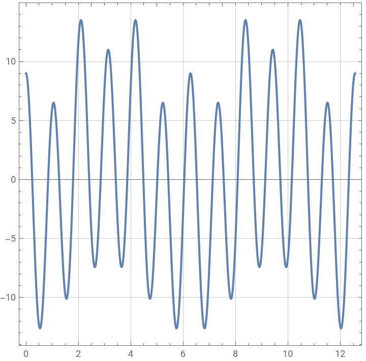
ILLUSTRATION 1 : sinusoidal signal without white noise
ILLUSTRATION 1 : sinusoidal signal without white noise
In[]:=
f[x_]:=-3Cos[x]+2Cos[3x]+10.0Cos[6x]
In[]:=
Plot[{f[x]},{x,0Pi,4Pi},PlotStyleThick,FrameTrue,GridLinesAutomatic,AspectRatio1]
Out[]=
In[]:=
data1=Table[Evaluate[f[x]],{x,0,50Pi,0.01}];dt=0.01;Ni=Length[data1]-1;omgmax=2*(Pi/dt);domg=omgmax/Ni;omg=Table[i,{i,0,omgmax,domg}];fdata=Abs[Fourier[data1,FourierParameters{1,1}]];tbl=Transpose[{omg,fdata/Max[fdata]}];
In[]:=
p={3,2,10.}/10.
Out[]=
{0.3,0.2,1.}
In[]:=
o={1,3,6}
Out[]=
{1,3,6}
In[]:=
points=Transpose@Join[{o,p}]
Out[]=
{{1,0.3},{3,0.2},{6,1.}}
In[]:=
p2=ListPlot[tbl,JoinedTrue,FrameTrue,GridLinesAutomatic,AspectRatio1,FrameLabel{Style["frequency",16,Italic],Style["power",16,Italic]},PlotRange{{0,10},{0,1.2}},PlotStyle{Brown,Thick},Epilog{PointSize[0.02],Darker@Blue,Point[points[[1]]],Point[points[[2]]],Point[points[[3]]]}]
Out[]=
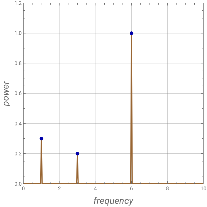
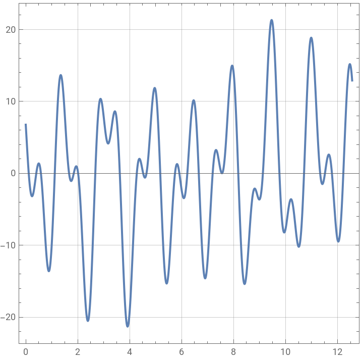
ILLUSTRATION 2 : sinusoidal signal without noise
ILLUSTRATION 2 : sinusoidal signal without noise
In[]:=
f[x_]:=-3.24Cos[3x]-2.14Sin[0.4x]+10.0Cos[4x]-7Sin[8.45x]
In[]:=
Plot[{f[x]},{x,0Pi,4Pi},PlotStyleThick,FrameTrue,GridLinesAutomatic,AspectRatio1]
Out[]=
In[]:=
data1=Table[Evaluate[f[x]],{x,0,1000Pi,0.01}];dt=0.01;Ni=Length[data1]-1;omgmax=2*(Pi/dt);domg=omgmax/Ni;omg=Table[i,{i,0,omgmax,domg}];fdata=Abs[Fourier[data1,FourierParameters{1,1}]];tbl=Transpose[{omg,fdata/Max[fdata]}];
In[]:=
p={3.24,10,2.14,7.}/10.
Out[]=
{0.324,1.,0.214,0.7}
In[]:=
o={3,4,0.4,8.45}
Out[]=
{3,4,0.4,8.45}
In[]:=
points=Transpose@Join[{o,p}]
Out[]=
{{3,0.324},{4,1.},{0.4,0.214},{8.45,0.7}}
In[]:=
p2=ListPlot[tbl,JoinedTrue,FrameTrue,GridLinesAutomatic,AspectRatio1,FrameLabel{Style["frequency",16,Italic],Style["power",16,Italic]},PlotRange{{0,10},{0,1.2}},PlotStyle{Brown,Thick},Epilog{PointSize[0.02],Darker@Blue,Point[points[[1]]],Point[points[[2]]],Point[points[[3]]],Point[points[[4]]]}]
Out[]=
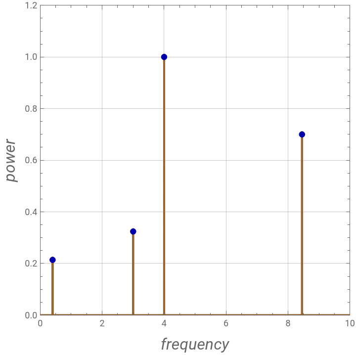
ILLUSTRATION 3 : sinusoidal signal with noise
One gets the same spectrum as illustration 1 however the baseline has noise.
ILLUSTRATION 3 : sinusoidal signal with noise
One gets the same spectrum as illustration 1 however the baseline has noise.
One gets the same spectrum as illustration 1 however the baseline has noise.
In[]:=
SeedRandom[1234]
In[]:=
data=Table[{x,-3Cos[x]+2Cos[3x]+10.0Cos[6x]+15RandomReal[{-1,1}]},{x,0,50Pi,0.01}]
Out[]=