Grid neural networks, which are neural networks arranged in a square grid, can be used to visualize the hidden layers in the networks while preserving regular capabilities of fully interconnected neural networks. In this paper, I explore the hypothesis spaces, which contain all approximable functions, and weight space, which contains all of the models’ weights. I conduct these tests through methods such as analyzing the random-sampled behavior of output curves, testing the ceilings for approximation of trained networks, and using principal component analysis to visualize patterns and effective dimensionalities of the weight spaces. I note that given neural networks trained on certain functions, their weight spaces form certain curves, whose behavior can be characterized through effective dimensionality and across h.
Introduction
Introduction
Neural networks approximate mathematical functions through the use of an activation function, which is applied to the output of the network to introduce non-linearity and drive proper function approximation. As the number of nodes and training rounds increases, the network’s parameters continuously adjust to get closer to the original function, capable of approximating to any desired degree. This idea is known as the Universal Approximation Theorem.
Per the Universal Approximation Theorem, models can theoretically form any continuous, differentiable function for approximation. This is done partially through increasing the complexity of the network. In traditional, fully interconnected neural networks, however, this expansion can be completed in two directions: layers and nodes, thus introducing further complications when analyzing metrics with increasing model size. This problem is addressed through the introduction of grid neural networks, as mentioned in the article “What’s Really Going On in Machine Learning? Some Minimal Models.” Grid neural networks have a diamond-like structure with equal side lengths, thus its size adjusts with only one variable.
Grid neural networks function by having at most two parents per neuron, which simplifies the structure and helps behavior visualization, like that of cellular automata, without significantly compromising function. Through exploring these networks and properly quantifying their possibilities, I characterize the internal structures of these grids.
I start this project through initializing the practical grid neural network and relevant functions, then exploring the minimal grid neural network. From this base, I explore the hypothesis spaces of the networks, as well as limits to that set. I then explore how the space changes with adjustments to complexity. From there, I address the inverse question of characterizing a given network’s multidimensional weight space. Lastly, I address potential limitations and future directions.
The Model
The Model
Grid neural networks typically possess a diamond-like shape:

Knowing this, I can define a few prerequisites.
Network Architecture
Network Architecture
To start, I define the diamond-shaped network architecture through a series of functions.
A row-width profile of the diamond structure:
In[]:=
diamondWidths[h_Integer]:=Join[Range[1,h+1],Range[h,1,-1]];
The total nodes and a helper to name node (r, c):
In[]:=
nodeName[r_,c_]:="n"<>ToString[r]<>"_"<>ToString[c];
Distinguish the interior nodes as the ones that carry weights:
In[]:=
interiorNodes[h_]:=Catenate@Table[{r,c},{r,2,Length@diamondWidths[h]},{c,1,diamondWidths[h][[r]]}]
Establish node parent wiring:
In[]:=
rowPositions[w_]:=Range[w]-(w+1)/2;
Define the parents of a node, distinguishing between top and bottom half:
In[]:=
parentsOf[widths_,r_,c_]:=With[{wPrev=widths[[r-1]]},Select[If[widths[[r]]>wPrev,{c-1,c},{c,c+1}],1<=#<=wPrev&]]
ELU Activation
ELU Activation
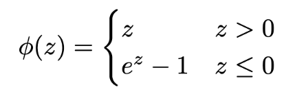
Next, I have to build the mesh as a NetGraph. Each node is a 2-input (1-input at edges) linear unit with the ELU (Exponential Linear Unit) activation function, as ReLU is not ideal for grid neural networks.
Mathematically, the ELU activation is piecewise, similar to ReLU:
Define activation function, ELU:
In[]:=
elu[z_?NumericQ]:=Which[z>0,z,z<-700.,-1.,True,Exp[z]-1]
Building the Mesh and Functions
Building the Mesh and Functions
Training is a key aspect in neural networks. A step-by-step process:
1
.I initialize the weights with the association nodeName -> {wL, wR, b}.
2
.Then, I establish forward pass. Given weights w and a scalar input x, I compute all node values top-to-bottom, then return the bottom node’s value.
3
.I define an input grid to build the sampled curve over.
4
.I train the model using Wolfram’s built in method, NetTrain.
Define the weight container:
In[]:=
initMeshWeights[h_,dist_:NormalDistribution[0,0.5]]:=Association[(nodeName@@#RandomVariate[dist,3]&)/@interiorNodes[h]]
Get scalar node value:
In[]:=
scalarNodeValue[widths_,w_,vals_,r_,c_]:=With[{nm=nodeName[r,c],pars=parentsOf[widths,r,c]},elu[w[nm][[1;;Length@pars]].(vals[nodeName[r-1,#]]&/@pars)+w[nm][[3]]]]
Get one row:
In[]:=
scalarRow[widths_,w_,vals_,r_]:=Join[vals,Association@Table[nodeName[r,c]->scalarNodeValue[widths,w,vals,r,c],{c,widths[[r]]}]]
Establish forward pass:
In[]:=
meshForward[h_,w_,x_]:=With[{widths=diamondWidths[h]},Fold[scalarRow[widths,w,##]&,Association[nodeName[1,1]->x],Range[2,Length@widths]][nodeName[Length@widths,1]]]
Build the input grid and grid-based curve:
In[]:=
grid=Range[0,1,0.005];meshCurve[h_,w_]:=Transpose@{grid,meshForward[h,w,#]&/@grid}
Define layers:
In[]:=
meshLayer[widths_,{r_,c_}]:=nodeName[r,c]->If[Length@parentsOf[widths,r,c]==1,NetChain@{LinearLayer[1],ElementwiseLayer["ELU"]},NetGraph[{CatenateLayer[],LinearLayer[1],ElementwiseLayer["ELU"]},{1->2->3}]]
Get parent indices for conversion:
In[]:=
meshPorts[r_,parents_]:=If[r-1==1,NetPort["Input"],nodeName[r-1,#]]&/@parents
Define edge of mesh:
In[]:=
meshEdge[widths_,{r_,c_}]:=With[{ports=meshPorts[r,parentsOf[widths,r,c]]},If[Length[ports]==1,First[ports],ports]->nodeName[r,c]]
Define trainable mesh:
In[]:=
meshTrainable[h_]:=With[{widths=diamondWidths[h],nodes=interiorNodes[h]},NetGraph[Association[meshLayer[widths,#]&/@nodes],meshEdge[widths,#]&/@nodes,"Input"->"Real"]]
I introduce some size bookkeeping metrics:
Map node to number of parents:
In[]:=
meshParents[h_]:=With[{widths=diamondWidths[h]},Association@Map[nodeName@@#->Length@parentsOf[widths,Sequence@@#]&,interiorNodes[h]]];
Flatten weight association into vector:
In[]:=
activeWeightVector[h_,w_]:=With[{parents=meshParents[h]},Catenate@KeyValueMap[If[parents[#1]==1,#2[[{1,3}]],#2]&,KeySort[w]]]
Get mesh parameter count:
In[]:=
activeMeshParamCount[h_]:=Length[activeWeightVector[h,initMeshWeights[h]]];
Now, I define the training function.
Define the train function:
In[]:=
trainMesh[h_,target_,rounds_:800]:=Module[{net,data},data=Table[x->{N[target[x]]},{x,grid}];net=NetInitialize@meshTrainable[h];NetTrain[net,data,MaxTrainingRounds->rounds,Method->{"SGD","Momentum"->0.8},LearningRate->0.005]]
Vectorized Functions
Vectorized Functions
For heavy processing and visualization, I define vectorized versions of the training functions to accelerate heavy computing:
Define vectorized ELU:
In[]:=
eluV=Map[If[#>0.,#,If[#<-700.,-1.,Exp[#]-1.]]&,#]&;
Find the value applied through a single node:
In[]:=
nodeValue[widths_,w_,prev_,r_,c_]:=With[{parents=parentsOf[widths,r,c],weights=w@nodeName[r,c]},eluV@Switch[Length[parents],1,weights[[1]]*prev[[First@parents]]+weights[[3]],_,weights[[1]]*prev[[First@parents]]+weights[[2]]*prev[[Last@parents]]+weights[[3]]]]
Find value across a row:
In[]:=
meshRow[widths_,w_,prev_,r_]:=Table[nodeValue[widths,w,prev,r,c],{c,widths[[r]]}]
Define vectorized forward pass:
In[]:=
meshVecForward[h_,w_,xs_List]:=With[{widths=diamondWidths[h]},First@Fold[meshRow[widths,w,##]&,{N[xs]},Range[2,Length@widths]]]
Apply new forward pass over the grid to return input->output pairs:
In[]:=
plotGrid=Range[0,10,0.005];
Apply mesh to trained NetChain/NetGraph:
All of the necessary functions to proceed are now defined.
Minimal Neural Networks
Minimal Neural Networks
I begin at the smallest nontrivial mesh, h = 1. Its diamond has widths {1, 2, 1}: one input, two hidden ELU nodes, and one output node. This is small enough to write in closed form and visualize.
The output is an explicit composition of ELUs. The seven active parameters can be written as p = {a1, b1, a2, b2, wL, wR, b}, with the two hidden units being g1 = ELU(a1 * x + b1) and g2 = ELU(a2 * x + b2).
Define the minimal network using ELU:
The minimal network has seven degrees of freedom:
Behavior Analysis
Behavior Analysis
Each hidden ELU activation is a monotone function, so the pre-activation of the output is a weighted sum of two monotone curves and a bias. The outer ELU is also monotone but cannot add extrema. As a result, the minimal network is essentially a monotone or single-turn family. I confirm this through random sampling networks and classifying their behavior through metrics:
Define the classify function:
Count minimum shapes:
Plot the table:
The distribution is dominated by monotone curves, with some single-extrema curves. Thus, the reachable set of the minimal network is a very narrow band, and this is because there is a small number of parameters, which limits how adjustable the output curve is. When expanding beyond minimal grid networks, patterns become more apparent.
Defining the Hypothesis Space
Defining the Hypothesis Space
With the new network architecture, I address the first core question:
For a fixed activation function, what shapes of functions does the network produce as you vary the weights?
For purposes involving grid neural networks, I am using ELU, as defined previously. Since ELU is smooth, the curves can be characterized using local extrema, monotonicity, output range, and overall roughness (derivative variation).
Defining Metrics
Defining Metrics
I start by defining the metrics through feature extraction on a smooth curve.
Number of local extrema:
Monotonicity (is there no extrema):
Output range on [0, 1]:
Roughness (variance in the second derivative):
Aggregating the features:
Family Catalog
Family Catalog
Now, I catalog the family based on the metrics. I plot a table that describes the metrics and a histogram that contains the distribution of extrema and roughness among randomly sampled curves of a fixed complexity.
Define family catalog function:
View h = 3 family qualities:
With relatively high monotonicity and low mean roughness, the curves produced when h = 3 are overall very simple.
View h = 10 family qualities:
When it comes to higher h values, such as h = 10, overall monotonicity decreases while extrema and roughness increases, producing less monotone and more chaotic curves.
Both histograms are strongly right-skewed, but the wider range present in h = 10 implies that the strong skewing can be attributed to the normal weight distribution, rather than the true capability of the net.
Training to Model Data
Training to Model Data
While randomly sampling gives an idea of the type of curves a model can produce, it is not an optimal indicator for testing a network’s true modeling capacity. I observe how a mesh can model in a complex manner by training a mesh to intersect a small point set, then overlaying the output with random-sampled curves for comparison.
Train a mesh to a set of points:
Define the family of trained functions:
Define a family of randomly sampled curves for comparison:
I create a plot that overlays the two types of curves, with interpolating outputs being thick blue curves and random outputs being thin and gray in the background.
Create the plot:
Generally, the trained neural nets strongly modeled the set of given points, while the randomly generated curves with the same complexity remained relatively monotone and smooth. Therefore, it can be assumed that the monotone behavior is caused by the distribution of the random weights, and grid neural nets with unrestrained complexity can approximate any set of data that produces a continuous and differentiable output function, as expected given the Universal Approximation Theorem.
Characterizing Unrepresentable Functions
Characterizing Unrepresentable Functions
From Defining the Hypothesis Space, ELU-based grid neural networks have a large hypothesis space given unconstrained size. However, this poses another question:
Can we characterize the functions that the network with a complexity constraint cannot represent?
Before starting computation, note that grid neural networks cannot approximate data sets that result in discontinuous or not differentiable output functions regardless of complexity, therefore these are not considered. Rather, I test the points at which a model with a set complexity fails, to mark the boundaries of the network’s capabilities.
Error Metric
Error Metric
I start by defining a function to train a fixed-size mesh to a target, which returns the trained net, its RMSE (loss), and the max pointwise error (Linf), which are used to characterize when the model starts to fail.
Define accuracy function:
Oscillation Ceiling
Oscillation Ceiling
The first ceiling to test is oscillation frequency; given sinusoids of increasing frequency, at what point does the RMSE of a grid neural network with fixed h start to climb? I label this point as the “oscillation ceiling” for the given mesh size, and I observe this by plotting model loss against increasing frequencies.
Plot RMSE vs. frequency:
Test with h = 10:
At a certain frequency, the RMSE rises sharply. In this case, the sharp rise occurs at x = 2, from which the error gradually increases.
Sharpness Ceiling
Sharpness Ceiling
The next ceiling to test is sharpness; given Gaussian curves of shrinking width, essentially approaching a spike, at what point does the high local curvature of the narrow bump become irreproducible by a fixed-size grid neural network? I label this point as the “sharpness ceiling.” I observe this by plotting model loss against the width of the Gaussian bump.
Plot RMSE vs. bump width:
Test with h = 10:
At x = 0.0005, there is a significant fall in RMSE, implying that the network starts to approximate the curve better at that point. Inversely, it can be concluded that as the bump variance shrinks to around 0.005, the loss starts to rise significantly, which characterizes the sharpness ceiling.
Overall, these metrics help visualize at what point a function becomes unrepresentable by a grid neural network, which helps narrow down the theoretical hypothesis space.
Failure Visualization
Failure Visualization
All models have a point of failure, but it is also important to note how the models fail. Using the sinusoidal and Gaussian models, I constrain the grid’s complexity and training duration to see the best approximation it attempted: how it failed. By defining a set of “hard target” functions then overlaying the model’s best attempt given constraints with it, I see what patterns the network followed in its attempts.
Define hard targets:
Create single attempt panel:
Loop attemptPanel[] through the list of failure targets for the gallery:
Here, the model significantly struggled with modeling sinusoidal curves as characterized by higher error, while it made somewhat recognizable attempts with the gaussian and step functions. High-frequency sinusoids have many steep frequent changes in curvature, which is difficult to model with these lower-complexity neural networks.
Thus, outside of the case of noncontinuous or nondifferentiable output functions, a grid neural network’s hypothesis space can be constrained through increasing the complexity of the target function, through methods such as increasing relative curvature and slopes.
Hypothesis Space Scaling
Hypothesis Space Scaling
Now that quantitative limits are defined for hypothesis spaces for fixed h, I explore the changes in the sets with growing network complexity. This “space” is technically indefinite, as neural networks can approximate infinitely many continuous smooth functions—however, the previous reproducible ceilings combined with the quantitative complexity metrics and approximation errors can be used to see how the possibilities expand.
The question:
How does a grid neural network’s hypothesis space scale with changes in its complexity?
Test Data Accuracy
Test Data Accuracy
Before the relevant functions, I introduce a testing aspect, to see how test accuracy scales with complexity as well. In order to accomplish this, I define a new grid and accuracy testing function. For the objectives, mesh node count correlates more accurately to model complexity than layer count, as parameters increase with the number of neurons.
Create distinct grid:
Establish mesh node count:
Define mesh test accuracy:
Now I can start testing how the space scales.
Changes in Space Ceiling
Changes in Space Ceiling
As noted previously, complexity ceilings rise with size, as introducing more parameters aids approximation. This change can be visualized by graphing best loss versus increasing sinusoid frequency. If points of sudden change move to the right or the rise in error becomes less sharp, the network has become more capable at modeling those sinusoids; the ceilings have fallen.
Shortly define oscillation curve:
Plot the oscillation ceiling graphs :
Generally, as h increases, the rise in RMSE becomes smoother, which implies that the model’s approximations of the higher-frequency sinusoids are improving.
Tracking Behavior With Complexity
Tracking Behavior With Complexity
As used in Defining the Hypothesis Space, there are quantitative metrics that can describe the complexity of network curves. For these purposes, I use extrema, roughness and monotonicity.
To track how the behavior of the curves changes with model size, I randomly sample curves for each mesh size, then plot mean extrema and monotonicity against node count. I also technically track mean roughness, but it is a more volatile value due to the nature of the second derivative in this context, so it is not graphed.
Get the random meshes:
Compute mesh curve statistics:
Get necessary statistics:
Get data by sweeping across complexities:
Create table with metrics:
Plot mean extrema vs. nodes:
Plot fraction monotone vs. nodes:
Actually get growth data:
Disregarding outliers, the “wiggliness” or mean extrema of the networks increases, while the monotonicity roughly decreases, showing that model complexity correlates to more complex shapes formed in random sampling, which requires a wider range of functions to happen. Therefore, model complexity positively correlates to the size of the hypothesis space.
Tracking Approximation Accuracy With Complexity
Tracking Approximation Accuracy With Complexity
The last metric works by measuring error on a single hard target over increasing complexity, then observing how RMSE, the loss, decreases as the function becomes representable.
Show this using a simple table and plot:
Here, as complexity increases, the neural network approximates curves better, and thus its hypothesis space expands.
To expand and see how the model reacts to data beyond the training set, I use the test accuracy metrics to plot test approximation error and accuracy versus model complexity.
Get test accuracy data:
Create accuracy table:
Plot error vs. complexity:
Plot test accuracy vs. complexity:
Excluding the first few data points, there are not many meaningful patterns within this data given the scale; the graphs are relatively constant after the first three data points, which suggest that after a certain level of complexity, increasing the model size does not have a significant effect on test-relevant results.
Mapping the Weight Space
Mapping the Weight Space
So far, I have thoroughly explored hypothesis spaces, but what about the inverse: weight spaces? To truly understand grid neural networks, it is key to understand the set of weights that characterize certain functions.
Given n weights of neural networks, their distribution in space is not chaotic or random; rather, the weights lie on a multi-dimensional manifold existing in n-dimensional space. This space of parameters is called the weight space. This leads to the primary question in this exploration:
For a specific input-output pair/set, where in the weight space does that mapping hold? What is interesting about the set?
Mesh Bank
Mesh Bank
In order to compare the behavior of trained weights to the general weights in the area, I first define the bank of randomly sampled curves.
Output curve & value at a certain point:
Create the bank using bankSample:
Single-Point Weight Space
Single-Point Weight Space
Next, I construct the single-point weight-space structure. The solution set is one scalar constraint on a P-dimensional weight space, so generally a (P-1)-dimensional surface. The solution set of a single input-output pair is represented as below:
While it is impossible to truly visualize, I can measure how the intersecting fraction scales and the local dimensionality via how the band pinches. Using principal component analysis (PCA), I create a plot which effectively summarizes the behavior of the weight space, ideally through modeling a curve, then observe its behavior.
Calculate number of solution hits:
Create helper function for solution hits calculation:
Create tolerance vs. number of hits table:
Flatten a given weight association into a fixed-order vector:
Collect randomly-sampled weight vectors that satisfy condition:
Use PCA to check clustering:
Note there is not much clustering happening currently; from this perspective, there is not much pattern in the weight space, as expected since the weights fall on a random distribution.
Trained Weight Space
Trained Weight Space
Randomly sampled neural networks that map one input -> output pair do not show much clustering or patterns. However, interesting patterns can be observed when the network is properly trained with stricter constraints on data.
First note how the solution set changes. Given k input-output pairs:
I proceed with the method.
Get node layer index:
Get node parameters:
Get node weights:
Define trained weight vector:
Obtain satisfying weights through training:
Adjust normal distribution to match satisfying weights for comparison:
Use PCA to plot the weights:
This plot of standardized interpolating weights models a curve. Now, I further analyze its properties.
Effective Dimensionality
Effective Dimensionality
For convenience, the set of weights is separated to input into functions.
Create weight set:
One way to analyze the weight space is through a metric known as effective dimensionality. Effective dimensionality quantifies the minimal number of independent degrees of freedom needed to describe the space.
The metric is calculated as a ratio of the eigenvalues of the space’s covariance matrix:
Get participation ratio:
Define effective dimensionality from covariance matrix:
Get set of valid vectors:
Compare effective dimensionality of weight space and null space:
As the effective dimensionality of the trained set is significantly lower than that of the null dimension, I note that for the data, interpolation plays a significant role in constraining the weight manifold. This is supported by the fact that generally, despite being in n-dimensional space, the manifold of weights rarely uses that number of dimensions; rather, it compresses the space down into the dimensions that contain meaningful patterns. This is what effective dimensionality quantifies.
Weight Space Visualization of Common Functions
Weight Space Visualization of Common Functions
I conduct the same test with a variety of common functions, seeing what patterns form in the weight spaces. This is done by creating a PCA projection like before for each function, where the set of points to be used as data to interpolate is randomly sampled from a given range and effective dimensionality is calculated per each panel.
Gather common functions:
Split projection vectors:
Project vectors using PCA:
Sample points from PlotGrid to interpolate:
Get data for panel:
Draw panel w/ effDim data:
Actually make panel:
Build the whole gallery of PCA-based weight plots:
Note: The gallery takes a significant amount of time to evaluate.
Here, the constraints on simpler targets, such as polynomial and sigmoid, force the weight space into essentially a one-dimensional curve, while more complicated functions, such as log and sine have more multidimensional structure.
Analyzing Weight Significance
Analyzing Weight Significance
Now that weight spaces have been viewed in a static context, it can be analyzed how changing them affects neural network outputs.
One way to analyze the effect of change is using a neural network’s parameter Jacobian matrix. In backpropagation, models use the parameter Jacobian to view how small changes in the weights affect the overall output. For a neural network with m outputs and n learnable parameters, the Jacobian is a m x n matrix of partial derivatives.
Grid neural networks have one output, meaning in this case, parameter Jacobian takes the form:
where y represents the output, w the weights, and b the biases.
While this is interesting, eigenvalues are not defined for row matrices; I convert the Jacobian into a square matrix. This is done by using a “pullback metric” matrix G, which is simply the transpose of the Jacobian multiplied by the original.
The pullback metric measures distances in weight space as felt in function space; if a weight is slightly adjusted and the output curve changes significantly, it has a large value, and vice versa. By analyzing the eigenvalues of the matrix, I determine which weights are significant in changing the output of the neural net.
Create a column for the Jacobian:
Define the Jacobian matrix:
Define pullback metric:
Eigenvalue Spectrum
Eigenvalue Spectrum
Since the effective dimensions of the tested curves are close to 1, I hypothesize that the pullback metric is dominated by one eigenvalue. Thus, the effect of adjusting weights can be visualized as a ListLogPlot of eigenvalues vs. index.
Define eigenvalue spectrum:
I see that the first eigenvalue is vastly greater than the others (the difference between the first and second index is around five orders of magnitude), matching the hypothesis. Therefore at a random weight point, moving the weights only changes the output function along essentially one direction. The other 44 have significantly smaller eigenvalues, thus contribute much less.
Local Dimension Analysis
Local Dimension Analysis
Now, I use the participation ratio to get an effective local dimension of the function manifold. Tracking that effective dimension against h, and against the position on the solution set, is where the patterns lie.
Calculate local effective dimension:
Calculate mean effective dimension:
Get data over a range of h:
Plot mean effective dimension vs. total nodes:
As model complexity rises, the mean effective dimension decreases, practically converging to 1. This suggests that as a grid neural network grows in size, the effective dimensionality of its weight space converges to 1, so the pullback metric becomes more and more dominated by one eigenvalue.
Conclusion
Conclusion
In this paper, I explored many qualities of the hypothesis and weight spaces of grid neural networks. First, I defined a categorization method for ELU-based grid neural network output curves with quantitative metrics and explored their sampled and trained behavior. Then, I tested the boundaries of failure for these neural networks with example functions and have found at what points, given limited complexity and training, a model fails to model a continuous, differentiable function. After , I explored how scaling grid neural network size affects the hypothesis space and overall accuracy. Then, translating to the inverse question, I mapped the weight space of neural networks whose weights satisfy the interpolation constraints using principal component analysis, and have noted that the effective dimensions for the vast majority of these curves lies between 1 and 1.5, with many closer to 1. With this, I used the “pullback metric” calculated using the parameter Jacobian matrix and analyzed the effects of adjusting weights on the overall weight space, finding that in random-initialized meshes, only one eigenvalue tends to be very significant. Lastly, I found that effective dimensionality decreases with increasing complexity, suggesting that larger networks are more degenerate.
Limitations:
Limitations:
◼
Effective dimensionality alone does not fully characterize the behavior of the weight space.
◼
The methods and results described strictly apply to ELU-based grid neural networks; it does not generalize.
◼
Computation of multiple trials of complex functions involving neural net training such as pcaGallery[] takes excessive amounts of time, which makes finding true patterns difficult.
Future Directions:
Future Directions:
◼
Predict a solution manifold’s dimension and orientation from architecture without sampling.
◼
Generalize the activation beyond ELU.
◼
Explore how the defined metrics behave when extended to other network structures such as MLP.
Acknowledgments
Acknowledgments
I would like to thank Stephen Wolfram for suggesting this project. I also would like to express a great thanks to Junseo Lee, my mentor, for guiding me and helping me greatly in the process. I would also like to thank Lusine Sukiasyan, my advocate, for guiding me through my explorations of the Wolfram environment. Lastly, I want to thank the WSRP directors, Megan, Eryn, and Rory, as well as Bryan Chen, my awesome TA, who made this program an amazing experience for me and my peers.
References
References
Han, X., Wang, Z., Zhao, B., Zhang, B., Li, J., Borth, D., Yu, R., Maron, H., Ye, Y., Yin, L., & Neri, F. (2026). A survey of weight space learning: Understanding, representation, and generation (arXiv:2603.10090). arXiv. https://arxiv.org/abs/2603.10090
Szymanski, L., McCane, B., & Albert, M. (2018). The effect of the choice of neural network depth and breadth on the size of its hypothesis space (arXiv:1806.02460). arXiv. https://arxiv.org/abs/1806.02460
Wang, R., Xu, Y., & Yan, M. (2024). Hypothesis spaces for deep learning (arXiv:2403.03353). arXiv. https://arxiv.org/abs/2403.03353
Wolfram, S. (2024, August 22). What’s really going on in machine learning? Some minimal models. Stephen Wolfram Writings. https://writings.stephenwolfram.com/2024/08/whats-really-going-on-in-machine-learning-some-minimal-models/
Wurgaft, D., Rager, C., Kowal, M., Shyam, V., Feucht, S., Bhalla, U., Haklay, T., Bigelow, E., Sarfati, R., McGrath, T., Lewis, O., Merullo, J., Goodman, N., Fel, T., Geiger, A., & Lubana, E. S. (2026). Manifold steering reveals the shared geometry of neural network representation and behavior (arXiv:2605.05115). arXiv. https://arxiv.org/abs/2605.05115
Liang, C. (2025, July 11). Analyzing neural networks with mathematical modeling. Wolfram Community. https://community.wolfram.com/groups/-/m/t/3502213
CITE THIS NOTEBOOK
CITE THIS NOTEBOOK
Characterizing the hypothesis and weight spaces of grid neural networks
by Jason Eun-Shik Tae
Wolfram Community, STAFF PICKS, July 9, 2026
https://community.wolfram.com/groups/-/m/t/3751710
by Jason Eun-Shik Tae
Wolfram Community, STAFF PICKS, July 9, 2026
https://community.wolfram.com/groups/-/m/t/3751710