I use the minimal example that exhibits contextuality—the KCBS pentagon—to build a graph state by gluing the pentagons together in different ways. I quantify the quantum advantage of the state from input-output statistics alone using the gap density, and ask which configuration gives the highest quantum advantage.
The results: a novel representation-theoretic framework for quantum certification, framing the KCBS pentagram as a fundamental decision-theoretic unit to distinguish between classical, quantum, and post-quantum physical models.
The results: a novel representation-theoretic framework for quantum certification, framing the KCBS pentagram as a fundamental decision-theoretic unit to distinguish between classical, quantum, and post-quantum physical models.
Introduction
Introduction
Quantum mechanics predicts correlations between measurement outcomes that no classical device can fully replicate — a genuine, provable advantage, and the target of ever more sophisticated classical methods that try to imitate it. Its cleanest demonstration is the CHSH game, defined and quantified later in this chapter: two isolated players who share an entangled state win more often than any classical strategy — however clever, and with however much shared randomness — can. This gap, in its most general form called contextuality, is the resource the rest of this essay is built on. Before developing the methods, we walk through each of the fundamental terms, with definitions that give us a solid base for the more advanced reasoning without getting lost along the way. This will ultimately lead us to criteria for answering the following question:
Given only a device’s input–output statistics, can its interior be certified as genuinely quantum-mechanical, rather than built from classical parts?
Out[]=
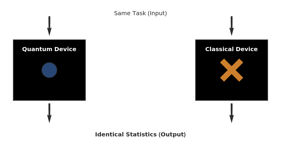
To answer this question, we focus first on the most fundamental phenomenon separating classical from quantum mechanics.
Quantum Entanglement
Quantum Entanglement
To define what “quantum entanglement” means in this essay, it is best to start from its observable consequences, framed by what is known as the EPR paradox. Einstein, Podolsky and Rosen (1935) noticed that quantum mechanics allows two systems (e.g. particles), once entangled, to show correlations between their separate measurement results so strong that predicting one system’s outcome seems to require instantaneous knowledge of what happens to the other, however far apart they are. Their proposed resolution was that quantum mechanics must be an incomplete description of a deeper, local, realistic theory — one where every outcome is fixed in advance by some (possibly hidden) variable, while no information is processed faster than the speed of light. Bell (1964) made this philosophical claim mathematically precise, and falsifiable: any theory in which outcomes are fixed by shared hidden variables, with no signal exchanged between the parties, must obey a specific inequality, testable in what is now called a Bell test.
The easiest way to picture what follows — using a concept Bell did not yet have — is the qubit: the smallest quantum system, with two distinguishable basis states, written |0⟩ and |1⟩. A general qubit state is a superposition α|0⟩ + β|1⟩ with |α|² + |β|² = 1, drawn as an arrow on a sphere: |0⟩ at the north pole, |1⟩ at the south, superpositions in between. Every single-qubit gate is a rotation of this arrow, and a measurement in the {|0⟩, |1⟩} basis returns 0 with probability |α|² — so rotating a qubit continuously reshapes its outcome statistics:
Out[]=
 |
θ=0: |0⟩ |
 |
θ= π 4 π 8 π 8 |
 |
θ= π 2 0⟩+1⟩ 2 |
The middle panel is worth remembering: its amplitudes are cos(π/8) and sin(π/8), and the square cos²(π/8) ≈ 0.854 will return later in this chapter as the agreement probability that CHSH turns into a witness.
In matrix form, the two basis states are column vectors:
In matrix form, the two basis states are column vectors:
Out[]=
,
1 |
0 |
0 |
1 |
The Hadamard gate H is the rotation taking the north pole to the equator — |0⟩ to the equal superposition (|0⟩+|1⟩)/√2:
Out[]//MatrixForm=
1 2 | 1 2 |
1 2 | - 1 2 |
The controlled-NOT acts on two qubits at once: on the basis {|00⟩, |01⟩, |10⟩, |11⟩} it flips the second (target) qubit exactly when the first (control) is |1⟩ — the ingredient that ties two qubits together:
Out[]//MatrixForm=
1 | 0 | 0 | 0 |
0 | 1 | 0 | 0 |
0 | 0 | 0 | 1 |
0 | 0 | 1 | 0 |
The act of preparing entanglement between two systems can be visualized with the Wolfram Quantum Framework: a Hadamard, then a controlled-NOT, applied to two qubits starting at |00⟩ — the standard Bell-pair preparation, drawn natively:
Out[]=
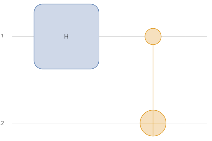
Apply it, and check genuine entanglement directly through validating whether that state cannot be written as a product of two independent systems:
Out[]=
True
Philosophical and mathematical constraints, unfortunately, do not always translate into something realizable in a laboratory. Because Bell’s original proposal was hard to deliver experimentally, an operational version was developed — due to Clauser, Horne, Shimony and Holt (1969), and referred to hereafter as CHSH — which serves as the primary metric for entanglement in the rest of this essay.
CHSH
CHSH
The basic building block of this concept is correlator E(a, b), defined for a fixed settings of measurements (a, b), where E acts as the expectation value ⟨A·B⟩ of the product of these two ±1 outcomes over repeated runs of sourcing and measuring particle’s polarization; since the product of a single run measurement is +1 on agreement and −1 on disagreement between pairs, correlator score is E(a, b) = P(same) − P(different) ∈ [−1, +1]. At the setting of a single correlator, quantum mechanics predicts E(a₀, b₀) = +:
1
2
Out[]=
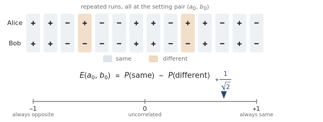
The measurement statistics themselves bring the real content. Classically, perfect correlation comes from a strategy where both sides always answer +1 which makes every setting pair agree, so all four correlators reach 1 — but for any assignment of predetermined answers the product of the four correlators is necessarily +1, so if three of them are perfect the fourth is forced to +1 as well, and the minus sign in S caps the total at 2. Quantum mechanics does what no such assignment can: three settings agree with probability cos²() ≈ 0.854 (correlator +), while the fourth disagrees just as strongly (correlator −) — each individually weaker than the classical +1, but carrying the one sign flip that pushes the sum to :
π
8
1
2
1
2
2
2
Out[]=


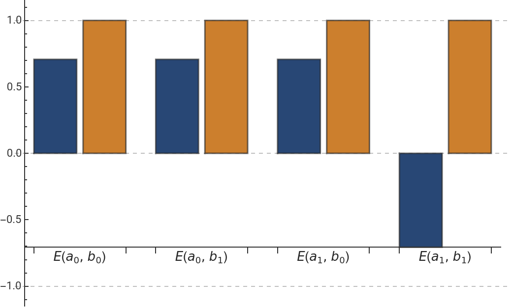
Now read off the four correlators at the settings that saturate CHSH — Pauli Z and X for Alice, their ±45° rotations for Bob — and combine them.
Out[]=
,,,-
1
2
1
2
1
2
1
2
In total, four correlators form the combination S = E(a₀,b₀) + E(a₀,b₁) + E(a₁,b₀) − E(a₁,b₁). Every local hidden-variable theory obeys |S| ≤ 2, while quantum mechanics, given an entangled pair and the right measurement settings, reaches S = ≈ 2.828 — Tsirelson’s bound (Tsirelson, 1980). True entanglement is therefore demonstrated explicitly by violating the classical bound through encountering statistics of events:
2
2
Out[]=
2
2
CHSH Game and beyond
CHSH Game and beyond
The same violation can be recast as a game — the form in which CHSH is usually run in the literature on Device-Independent applications (such as some Quantum Key Distribution protocols). A referee sends independent random bits x to Alice and y to Bob; each answers a bit, with no communication allowed once play begins; they win if their answers satisfy a ⊕ b = x ∧ y, the AND of the questions. Classically, the best they can do is agree beforehand on a joint strategy, possibly using shared randomness (a “hidden variable”) — and every such strategy wins at most of the time. Sharing an entangled pair instead lets them win with probability () = ≈ 0.854: winning means agreeing on three of the four question pairs and disagreeing on the fourth, so the win probability is exactly the per-setting agreement probability computed above. The ceiling and |S| ≤ 2 are the same classical fact in different units, just as 0.854 and S = are different representations of the same quantum mechanical invariant.
3
4
cos²
π
8
(2+
2
)4
3
4
2
2
Classical bound, Tsirelson’s bound, and the gap between them:
Out[]=
,,0.1036
3
4
2
Cos
π
8
CHSH needs two ingredients at once to beat the game’s classical ceiling: entanglement, and distance. The distance is what enforces the no-signaling condition: light travels about 30 cm per nanosecond, so when the two stations are a kilometer apart and each finishes its measurement within a microsecond, no signal — even at light speed — can pass between them in time; any advantage beyond the classical ceiling can therefore come only from the shared quantum state. But is this pair of ingredients the only way to rule out the pre-assigned measurement outcomes posited by hidden-variable theories? Kochen and Specker (1967), and later Klyachko, Can, Binicioğlu and Shumovsky (2008), showed that it is not. A single quantum system — one qutrit, measured in sequence, with no partner anywhere — also produces statistics that no table of pre-assigned answers can reproduce. Proving this requires exactly two assumptions about such a table: that it exists at all — every observable has a definite value waiting to be read out (value definiteness) — and that each value is independent of which other, compatible measurements are performed alongside it (noncontextuality). The set of accompanying compatible measurements is called the context; the failure of noncontextuality is contextuality. Locality is one way of guaranteeing noncontextuality: in a Bell test, the other measurement in the context is precisely the one performed at the distant station, and if the local outcome depended on it, that dependence would be a faster-than-light influence — exactly what the separation forbids. So when the statistics nonetheless overshoot the classical bound, what has failed is precisely the independence from context. Nonlocality is therefore the special, spatially separated case of contextuality.
Quantum Contextuality
Quantum Contextuality
If contextuality is the general resource, the natural next question is: what is the smallest system in which isolating it is possible? The original Kochen–Specker argument is a logician’s object — 117 projection directions in dimension three, colored into a contradiction. It rules out non-contextual value tables, but as an experiment, similarly as Bell test, it is hopeless: the contradiction is exact only for perfectly aligned measurements, and any finite imprecision blurs it away. What Klyachko, Can, Binicioğlu and Shumovsky concluded from it is the minimal testable framework: five binary measurements, arranged in a 5-element cycle (pentagram) so that neighbors are compatible and mutually exclusive, known as KCBS pentagram.
◼
Exclusivity Graph (Principle)
◼
Independence Number α(G)
◼
Lovász Number ϑ(G)
◼
Fractional Packing Number α*(G)
The language that makes this precise — and the reason the pentagon is the right building block for constructing graph states — is the Exclusivity Principle, which assigns one vertex per measurement event, and one edge per pair of events that are mutually contradictory, e.g. can never both occur at the same time. In this representation the reach of each physical theory becomes a computable graph invariant, so the physics of a contextuality experiment reduces to graph theory.
Why the angle is forced: sweeping the cone, the handle-state click rate (blue) changes smoothly and singles out nothing, while the crosstalk — v₊₁ firing right after vₖ, which exclusivity requires to be exactly zero — vanishes only at θ*. A 5° tilt already yields 2.5% forbidden co-clicks: the finite-precision sensitivity that long kept Kochen–Specker-type constructions out of the lab, and that any real KCBS test must budget for.
All five adjacent dot products vanish identically and every direction is a unit vector — the C₅ exclusivity edges are realized exactly:
An interesting question that may come in mind when observing described dynamics is why exactly pentagon work best as a model for contextuality, given the fact that each observable is dichotomic, and orthogonal neighbors force joint measurability, so a cycle of any length is potentially available to test geometrical relations.
Even though cycles saturate the bound between classical and quantum-mechanics, its smallest form, C3, don’t hold a proof for it: three mutually orthogonal directions in a 3-dimensional Hilbert space form a single shared context, so no contextuality can appear. C5 is the smallest cycle where this collapse does not happen — therefore it is the genuine atom of contextuality.
Even though cycles saturate the bound between classical and quantum-mechanics, its smallest form, C3, don’t hold a proof for it: three mutually orthogonal directions in a 3-dimensional Hilbert space form a single shared context, so no contextuality can appear. C5 is the smallest cycle where this collapse does not happen — therefore it is the genuine atom of contextuality.
Measurement result over each KCBS projector on the handle state through QuantumMeasurementOperator:
KCBS delivered experimentally
KCBS delivered experimentally
Lapkiewicz et al. (2011) realized KCBS with a single heralded photon distributed over three optical modes — an actual qutrit — reconfiguring one apparatus through five wave-plate settings so that the setup measuring the observable shared between neighboring contexts is left physically untouched, enforcing compatibility by construction along the chain. Only the pentagon’s closing edge resists this: there the experiment measures a sixth observable A₁′ in place of the original A₁ and tests an extended inequality with a measured correction term 1 − ⟨A₁A₁′⟩ accounting for the difference.
◼
heralded single photon
The apparatus, schematically: one heralded photon spreads over three optical modes — drawn here as three paths, with |0⟩, |1⟩, |2⟩ labeling which mode is occupied (in the actual experiment two of the modes were the two polarizations of a single beam). The modes are the qutrit. The blue plates φ stand for the wave-plate settings that select which commuting pair of KCBS directions — which measurement context — is tested, so all five contexts are five settings of this one interferometer, recombined onto the detectors D. Along the chain of contexts the shared measurement keeps the same optics and the same detector, enforcing compatibility by construction; the pentagon’s closing edge cannot be enforced this way and is handled by a sixth measurement A₁′ with a measured correction term:
◼
unitary operator / unitarity
This closes the audit of the atom: one pentagon, three ceilings, separated in theory, computed live, and pinned by experiment. Everything that follows asks what this atom can build — take several pentagons, let neighbors share a detector, and watch what gluing does to the three ceilings. That is the subject of the next section.
Manipulating and Composing Pentagons
Manipulating and Composing Pentagons
◼
orthogonal group O(3)
Apply each joint type to the pentagon’s own vertex labels: direct rotates 0→1→2→3→4→0 (determinant +1); twisted reflects across the axis through vertex 2, fixing it and swapping 0 with 4, 1 with 3 (determinant −1):
Both operations act on a genuine physical qutrit — the same three-dimensional system the KCBS pentagon already lives in — so they compose as an actual quantum circuit.
Both single-qutrit gates are confirmed unitary by the framework itself, and the assembled three-gate circuit’s own matrix has determinant −1 — exactly, since determinants multiply: two rotations compose to a rotation, and the one reflection flips the overall parity. This is the same fact, now checked as an actual gate sequence rather than argued combinatorially, that makes a single twisted joint irreducible while two consecutive ones partially cancel — the intuition behind why ddt (isolated flips) beats pure twisted (paired flips):
Spot-check the representation witness at four odd N — cyclic orthogonality (including wrap-around), unit norm, and the value identity all verified live:
The matching α bound comes from counting: every pentagon induces its own five-cycle (independence number 2), and summing this window bound over all N pentagons counts each glue’s shared vertices twice and its free vertex once, giving 2·(shared) + (free) ≤ 2N and hence α ≤ ⌊3N/2⌋; the alternating set of every free vertex plus every other rail vertex attains it. For even N this already forces ϑ = α = α* = 3N/2 exactly — no possible gap, at any level of the hierarchy.
The contrast plotted — bounded versus linear:
The curve that keeps climbing is the twisted ring — its peaks grow in proportion to N, extensive by the proof above, even though it dips whenever N is a multiple of 3. The curve pinned to exactly zero at every even N and creeping toward 1/2 at odd N is the direct ring, bounded by the same proof — neither curve’s shape is incidental.
Searching for the Optimal Word
Searching for the Optimal Word
Build an open ribbon of the ddt mesh — eight ddt periods, 25 pentagons; a block is drawn mirrored exactly when an odd number of twisted joints precede it:
All four checks hold: the 51-gate circuit is unitary, its net determinant is exactly −1 (17 twisted joints, an odd number), and both independent cross-checks match the raw product exactly — the drawn mirror pattern, the algebraic unit-cell power, and the actual quantum circuit are three views of the same computation, not three separate claims.
Measured as the quantum advantage contributed per pentagon (the gap density), the three strategies compare as follows:
Why This Search Resists a Proof
Why This Search Resists a Proof
Build the de Bruijn-3 graph over {d,t}, highlighting the ddt orbit:
Why ddt is special among periodic orbits — and why nothing simpler detects it. A periodic gluing orbit is a repeating word over {d, t}, and its ϑ-density is the per-block limit of ϑ along the rings it builds. (A) the spectrum of these densities: it runs from the twisted ring’s τ* ≈ 1.3767 at the bottom to the direct ring’s 3/2 at the top, with mixed orbits — 16/11, 19/13, 25/17, … — crowding a narrow band just beneath the ceiling. On this axis ddt itself, at 1.40323, sits low and looks entirely unremarkable: raw ϑ-density cannot single it out, because the orbits that earn the most ϑ also pay the most on the classical side — what matters is the difference, and panel A never sees the classical side at all. (B) the same orbits through the policy-iteration lens of ergodic optimization: the value the iteration assigns to each seeding orbit, plotted against that orbit’s density. Every spurious fixed point — an orbit at which the iteration stalls without being optimal — lands on the common line value = density − 1; the true optimum alone drops by a further 1/3 to the line value = density − 4/3, its offset being exactly the classical floor ᾱ = 4/3 that ddt uniquely achieves at maximal direct fraction. Its value coordinate there is 1.40323 − 4/3 = 0.0698975 — the gap density itself, read directly off the plot rather than asserted. The two panels together are the point: the quantity being optimized is invisible to the spectrum alone and becomes a straight-line diagnostic only when the classical floor enters:
Why the limit, and not a finite mesh? A finite mesh yields only a partial average, and its value drifts with where the reading stops. Only the n → ∞ limit is a property of the pattern itself rather than of an arbitrary cutoff — and a larger limit means more quantum advantage retained per pentagon as the mesh grows. That single number is exactly what the certificates above bound across all gluing words at once, and why gap(ddt) = 0.0699 is the value to beat.
Concluding Remarks
Concluding Remarks
The Ceiling and the Floor
The Ceiling and the Floor
Two facts hold for every gluing word at once, periodic or not, and together they close most of the gap left open above. The first is a hard ceiling: no choice of word can push ϑ̄(W) above 3/2. The proof is a single accounting assignment read two ways. Spreading weight 1/2 over each block’s two internal edges and two glue-in edges (leaving the shared edge bare) yields a fractional clique cover of value 3/2 per block, so ϑ̄(W) ≤ 3/2; spreading weight 1/2 over every vertex instead yields a fractional packing of the same value, so by LP duality the bound is exact.
Put the ceiling and the floor together and the open question shrinks to a narrow strip:
Future Directions
Future Directions
Three directions follow directly from the boundary of what is proven above.
◼
Rule out, or find, an aperiodic competitor. Since the finiteness property of ergodic optimization can fail — admitting a non-periodic (Sturmian) maximizer — the natural next step is a targeted search or exclusion argument over aperiodic gluing words, rather than further periodic enumeration.
Codebase
Codebase
All computations behind the results presented here are available in the author’s repository, https://github.com/hubertkolcz/BlackBox, and every figure and certificate can be reproduced from there.
Acknowledgments
Acknowledgments
The author thanks Nik Murzin, Pavel Hajek, Xerxes Arsiwalla, and Stephen Wolfram for guidance on this research thread. Computational and drafting assistance from generative AI is disclosed in AI Disclosure below.
References
References
1
.Einstein, A., Podolsky, B., & Rosen, N. (1935), “Can Quantum-Mechanical Description of Physical Reality Be Considered Complete?” Physical Review, 47(10), 777–780.
2
.Bell, J. S. (1964), “On the Einstein Podolsky Rosen Paradox,” Physics Physique Fizika, 1(3), 195–200.
3
.Kochen, S., & Specker, E. P. (1967), “The Problem of Hidden Variables in Quantum Mechanics,” Journal of Mathematics and Mechanics, 17(1), 59–87.
4
.Clauser, J. F., Horne, M. A., Shimony, A., & Holt, R. A. (1969), “Proposed Experiment to Test Local Hidden-Variable Theories,” Physical Review Letters, 23(15), 880–884.
5
.Lovász, L. (1979), “On the Shannon Capacity of a Graph,” IEEE Transactions on Information Theory, 25(1), 1–7.
6
.Tsirelson, B. S. (1980), “Quantum Generalizations of Bell’s Inequality,” Letters in Mathematical Physics, 4(2), 93–100.
7
.Bousch, T., & Mairesse, J. (2002), “Asymptotic Height Optimization for Topical IFS, Tetris Heaps, and the Finiteness Conjecture,” Journal of the American Mathematical Society, 15(1), 77–111.
8
.Klyachko, A. A., Can, M. A., Binicioglu, S., & Shumovsky, A. S. (2008), “Simple Test for Hidden Variables in Spin-1 Systems,” Physical Review Letters, 101(2), 020403.
9
.Lapkiewicz, R., Li, P., Schaeff, C., Langford, N. K., Ramelow, S., Wiesniak, M., & Zeilinger, A. (2011), “Experimental Non-Classicality of an Indivisible Quantum System,” Nature, 474(7352), 490–493.
10
.Cabello, A. (2013), “Simple Explanation of the Quantum Violation of a Fundamental Inequality,” Physical Review Letters, 110(6), 060402.
11
.Cabello, A., Severini, S., & Winter, A. (2014), “Graph-Theoretic Approach to Quantum Correlations,” Physical Review Letters, 112(4), 040401.
12
.M. Ulrey (2022), “The role of (non)contextuality in Bell’s theorems from the perspective of an operational modeling framework,” International Journal of Quantum Foundations, 8, 31–116.
Code Initialization
Code Initialization
AI Disclosure
AI Disclosure
The following generative AI tool was used in this project: Claude (Anthropic). It was used for restyling and regenerating figures from the author’s existing project artifacts, drafting narrative prose, and structuring this notebook to the Wolfram Summer Research Institute essay template and guidelines. All code and written content was reviewed, understood and approved by the author.
CITE THIS NOTEBOOK
CITE THIS NOTEBOOK
Evaluating Black-Box Physics Through Optical Emulation
by Hubert Kołcz
Wolfram Community, STAFF PICKS, July 16, 2026
https://community.wolfram.com/groups/-/m/t/3763738
by Hubert Kołcz
Wolfram Community, STAFF PICKS, July 16, 2026
https://community.wolfram.com/groups/-/m/t/3763738