This notebook is an update to three previous posts on the inverted yield curve:
FOMC raising rates: model for an inverted yield curve
FOMC rates: inverted yield curve is changing
Yield curve animation
The first post was made in November 2022 while interest rates were rising but before there was any stabilization to the yield curve shape. The second post was at the end of February 2023, when the yield curve began to show some signs of reverting, but before the market chaos created by bank failures and concern about the debt ceiling. The third post in March 2023, shows an animation of how the yield curve recovered in the 1980s. The current notebook adds a fifth parameter to the model which will now reasonably fit all the Treasury yield curves going back to the 1980s.
5-parameter model
5-parameter model
The new yield curve model uses a gamma distribution to replace the exponential distribution in the first model. When the k-parameter goes to 1, the model is the same as the initial model, which only worked for a special case of normally shaped yield curves.
In[]:=
CDF[GammaDistribution[k,1/a],t]//FunctionExpand%/.k->1CDF[ExponentialDistribution[a],t]//Simplify
Out[]=
|
Out[]=
|
Out[]=
|
In[]:=
yModel5=r0+(r-r0)1-Exp[-ct]UnitStep[t];
Gamma[k,at]
Gamma[k]
Below is the previous model.
In[]:=
yModel5/.k->1
Out[]=
r0+(1-)(r-r0)UnitStep[t]
-ct
-at
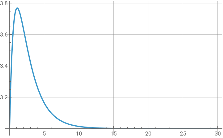
The Manipulate function shows how the shape of the yield curve changes with the parameters. The r0 and r parameters simply change the scale on the y-axis; the c-parameter is a measure of the degree of yield curve inversion. As c 0, the yield curve is no longer inverted. The a and k parameters control the location of the mode when the curve is inverted. When the yield curve is not inverted, c 0, the k parameter, k > 1, introduces an S-shape and the a-parameter controls the location of the inflection point. The S-shaped curve was observed during the financial crisis recovery, when the Fed manipulated the whole yield curve with “quantitative easing.”
In[]:=
ManipulatePlotr0+(r-r0)1-Exp[-ct]UnitStep[t],{t,0,30},PlotRange->All,GridLines->Automatic,{{r0,3},0,6},{{r,5},r0,8},{{k,1},0.01,5},{{a,1},0.02,5},{{c,0.5},0,3,0.01},SaveDefinitions->True
Gamma[k,at]
Gamma[k]
Out[]=


Yield curve data from the Treasury
Yield curve data from the Treasury
In[]:=
ycurves22=Import["https://home.treasury.gov/resource-center/data-chart-center/interest-rates/daily-treasury-rates.csv/2022/all?type=daily_treasury_yield_curve&field_tdr_date_value=2022&page&_format=csv","CSV"];ycurves23=Import["https://home.treasury.gov/resource-center/data-chart-center/interest-rates/daily-treasury-rates.csv/2023/all?type=daily_treasury_yield_curve&field_tdr_date_value=2023&page&_format=csv","CSV"];ycurves0=Join[ycurves23,Rest[ycurves22]];
The first row is the header, and the following rows are in reverse order by date.
In[]:=
yieldDS=AssociationThread[ycurves0[[1]],#]&/@Rest[ycurves0]/.""->Missing[]//Dataset
Out[]=


In[]:=
times=,,,,,1,2,3,5,7,10,20,30;
1
12
1
6
1
4
1
3
1
2
In[]:=
ycurves={DateObject[DateList[{#[[1]],{"Month","Day","Year"}}],"Day"],Transpose[{times,Rest[#]}]}&/@Reverse[Rest[ycurves0]]/.""->Missing[];
Data analysis and curve fitting
Data analysis and curve fitting
The fits are made only to the first ten years of the yield curve.
In[]:=
yModel5=r0+(r-r0)1-Exp[-ct]UnitStep[t];
Gamma[k,at]
Gamma[k]
In[]:=
Clear[yModel5Fn];yModel5Fn[t_,{r0_,r_,a_,k_,c_}]:=r0+(r-r0)1-Exp[-ct]UnitStep[t];Clear[modelCurve];modelCurve[data_]:=Module[{nlm,data1},data1=Select[Take[data,11],#[[2]]=!=Missing[]&];nlm=NonlinearModelFit[data1,{yModel5Fn[t,{Abs[r0],Abs[r],Abs[a],If[Abs[k]>10,8,Abs[k]],Abs[c]}]},{{r0,data1[[1]][[2]]/2},{r,2data1[[-1]][[2]]},{a,1},k,{c,0.5}},t];Association[#1->Abs[#2]&@@@nlm["BestFitParameters"]]];
Gamma[k,at]
Gamma[k]
In[]:=
alist={};Do[ya=Quiet@modelCurve[ycurves[[i]][[2]]];AppendTo[alist,Join[Association["date"->ycurves[[i]][[1]]],ya,Association["yieldCurve"->ycurves[[i]][[2]]]]],{i,Length[ycurves]}];//AbsoluteTiming
Out[]=
{10.0501,Null}
Parameter history and behavior
Parameter history and behavior
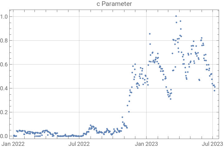
This plot shows the rapid rise of the c-parameter starting in October 2022. It seemed to be peaking in January 2023 then declining until the bank failures in March, when it again became chaotic until the debt ceiling was lifted. Recently it has begun a steady decline.
In[]:=
cdata={#["date"],#[c]}&/@alist;DateListPlotTooltip[#,#]&/@cdata,
Out[]=
This plot shows the c-parameter behavior since 31 May 2023, after the debt ceiling was resolved.
These plots show the behavior of the a and k parameters. The very high values after the bank failures most likely represent poor fits caused by fixed suggested fitting parameters in the NonlinearModelFit used in the modelCurve function. These parameters seem to have stabilized since May 2023.
Recent curve fit.
Recent weekly yield curve fits. Over this time frame, the FOMC has not changed rates so the change in the yield curve has been caused by market forces, including economic and inflation expectations. These will likely change with upcoming inflation data and FOMC meeting. Much of the rise in the tail of the curve also has to do with the recent rapid rise of the stock market.
Four week forecast based on c-parameter projection and the other parameters remaining stable.
It seems pretty unlikely that this forecast will hold with such a rapid rise in the ten year rate. It is possible for the shape prediction to be correct, but the scale parameters, r0 and particularly r, may not be stable.
For the projection above, the r0 parameter has been relatively stable, but the r parameter has been declining with the c-parameter, except for the most recent few points, taking the last point here will not likely be accurate, but projecting the decline since the end of May would bring the r-parameter below the r0-parameter and create a curve which would not be within the model.
Conclusion
Conclusion
The updated yield curve model now fits, reasonably well, all the Treasury data going back to 1990, and the FRED data going back to 1981. Earlier data in the FRED database may not have enough points on each yield curve to give a reliable fit to a five parameter model. When the Treasury market is chaotic the a and k parameters become anomalously high, but the c-parameter still carries useful information. Currently the yield curve evolution shows longer term rates rising more dramatically than shorter term rates. Whether the shape change is due to macroeconomic expectations or a slew of microeconomic factors is unclear, but the model is continuing to fit the first ten years of the of the curve as a smooth function. The c-parameter appears to be linearly declining now, but its past history shows that its path can easily be disrupted by market shocks. The section below shows the yield curve recovery from 1981 through 1982, the last time the yield curve became this significantly inverted. This notebook and the previously posted notebooks demonstrate how Mathematica can help visualize and analyze evolving data with a new model.
CITE THIS NOTEBOOK
CITE THIS NOTEBOOK
FOMC rates: inverted yield curve update with 5-parameters model
by Robert Rimmer
Wolfram Community, STAFF PICKS, July 7, 2023
https://community.wolfram.com/groups/-/m/t/2953857
by Robert Rimmer
Wolfram Community, STAFF PICKS, July 7, 2023
https://community.wolfram.com/groups/-/m/t/2953857