ABSTRACT (original article): We report new results on classical, Machian, fractons. For fractons of strictly bounded Machian range, we show that local clusters do not exhibit chaos while the global state breaks ergodicity. We show that the many fracton evolution characteristically exhibits a central time or Janus point and thus a generic non-equilibrium arrow of time as discussed previously in the context of classical Cosmology. CITATION (original article): Aryaman Babbar, Ylias Sadki, Abhishodh Prakash, S. L. Sondhi (2025), Classical Fractons: Local chaos, global broken ergodicity and an arrow of time, arXiv:2501.12445. https://doi.org/10.48550/arXiv.2501.12445
We set up the Hamiltonian for a system of n dipole conserving fractons. We assume that the fractons live on a 1 D line and have the same charge . In this regime, the centre of mass of the system is unchanged over time. In order to construct a translationally invariant, dipole conserving Hamiltonian for this system, we require that the Hamiltonian depends on position and momentum differences.
We then impose locality - which is to say that fracton pairs with large separation do not contribute to the Hamiltonian . If we consider the simplest possible quadratic Hamiltonian, this would have terms of the form and locality in this case is imposed by multiplying each such term with a “pair inertia” term, so each term in the Hamiltonian looks like . We use an exponentially decaying form of the pair inertia term for computations.
2
(-)
p
i
p
j
K(-)
x
i
x
j
2
(-)
p
i
p
j
Define the functions - Machian pair - inertia function, Hamiltonian and Complexity
ClearK;Cleareq1;Cleareq2;ClearinitialConditions;Clearsol;
Define the form of the Machian pair - inertia function that we will use
K[x_,η_]:=1/2*(Tanh[η*(x+1)]-Tanh[η*(x-1)]);
Each term in the Hamiltonian looks like this
hamiltonianFunction[q1_,p1_,q2_,p2_,η_]:=K[q1-q2,η]
1
2
2
(p1-p2)
Each term in the Complexity parameter looks like this
diffsq[p1_,p2_]:=1/2*(p1-p2)^2
Define the Hamiltonian for a system of N fractons
hamiltonian[p_List,q_List,η_]:=Sum[hamiltonianFunction[q[[i]],p[[i]],q[[j]],p[[j]],η],{i,Length[p]},{j,i+1,Length[p]}];
Complexity parameter - depends only on momenta
sumdiffsq[p_List]:=Sum[diffsq[p[[i]],p[[j]]],{i,Length[p]},{j,i+1,Length[p]}]
Hamilton’ s equations of motion
eq1[η_,n_]:=Table[D[q[i][t],t]==D[hamiltonian[Table[p[i][t],{i,1,n}],Table[q[i][t],{i,1,n}],η],p[i][t]],{i,n}];eq2[η_,n_]:=Table[D[p[i][t],t]==-D[hamiltonian[Table[p[i][t],{i,1,n}],Table[q[i][t],{i,1,n}],η],q[i][t]],{i,n}]initialConditions[Q0_List,P0_List]:=Flatten[Table[{q[i][0]==Q0[[i]],p[i][0]==P0[[i]]},{i,Length[Q0]}]]
Solve the equations
sol[η_,Q0_List,P0_List,n_,T_]:=NDSolve[Join[eq1[η,n],eq2[η,n],initialConditions[Q0,P0]],Flatten[Table[{q[i],p[i]},{i,n}]],{t,0,T}]
We let a system of n fractons time - evolve using Hamilton’ s equations of motion
eta=30;n=5;
Starts at t = 0 and runs till t = TT
TT=10;
Initial positions and momenta are randomly chosen
Qin1=RandomReal[{-0.5,0.5},{n}];Pin1=RandomReal[{-1,1},{n}];
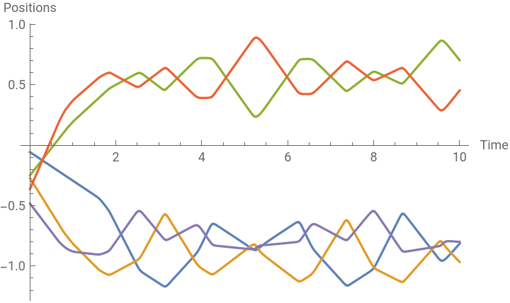
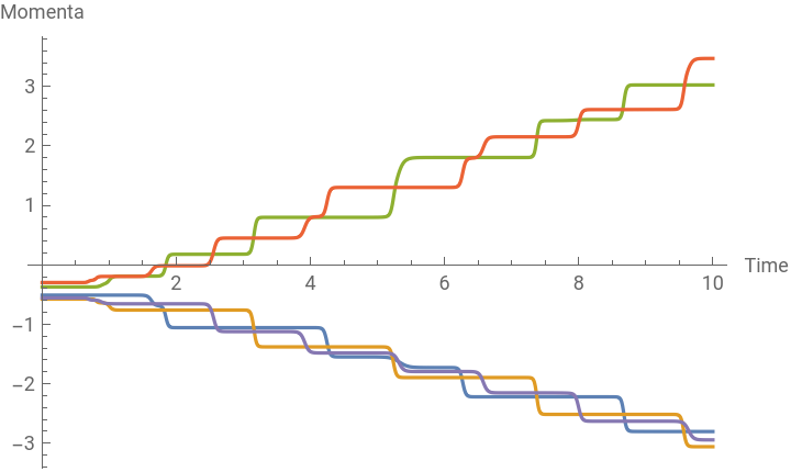
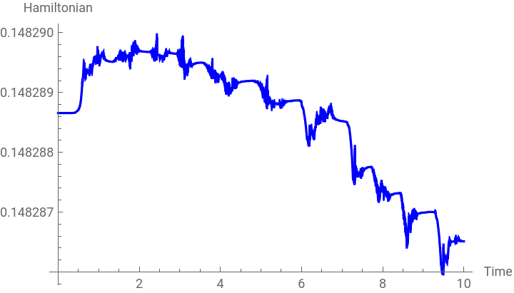
These plots show one of the most important aspect of fractonics dynamics - clustering . At later times, a system of n fractons always splits into more than one “Machian cluster” . Positions of centres of mass of clusters become constant at later times . Clusters are characterised by their centres of mass and by the fractons that make them . Clustering configuration sensitively depends on initial conditions and each such configuration corresponds to disjoint regions in phase space - hence, clustering leads to the breaking of ergodicity, which has other interesting consequences, such as the apparent breakdown of Mermin - Wagner theorem in small dimensions . The d = 1 case is illustrated in the plots below .
(*Plotthepositionandmomentumagainsttime*)Plot[Evaluate[Table[{q[i][s]}/.sol[eta,Qin1,Pin1,n,TT],{i,n}]],{s,0,TT},PlotLegends->Flatten[Table[{Subscript["x",ToString[i]]},{i,n}]],PlotRange->All,AxesLabel->{"Time","Positions"}]Plot[Evaluate[Table[{p[i][s]}/.sol[eta,Qin1,Pin1,n,TT],{i,n}]],{s,0,TT},PlotLegends->Flatten[Table[{Subscript["p",ToString[i]]},{i,n}]],PlotRange->All,AxesLabel->{"Time","Momenta"}](*PlottheHamiltonianagainsttimeforasanitycheck*)Plot[Evaluate[hamiltonian[Table[p[i][s],{i,n}],Table[q[i][s],{i,n}],eta]/.sol[eta,Qin1,Pin1,n,TT]],{s,0,TT},PlotRange->All,AxesLabel->{"Time","Hamiltonian"},PlotStyle->Directive[Blue]]
Out[]=


Out[]=
Out[]=
Complexity against time to show the presence of the Janus point for n fracton evolution
eta=40;n=5;
Plots complexity, position, momenta and Hamiltonian against time from t = -TT to t = TT
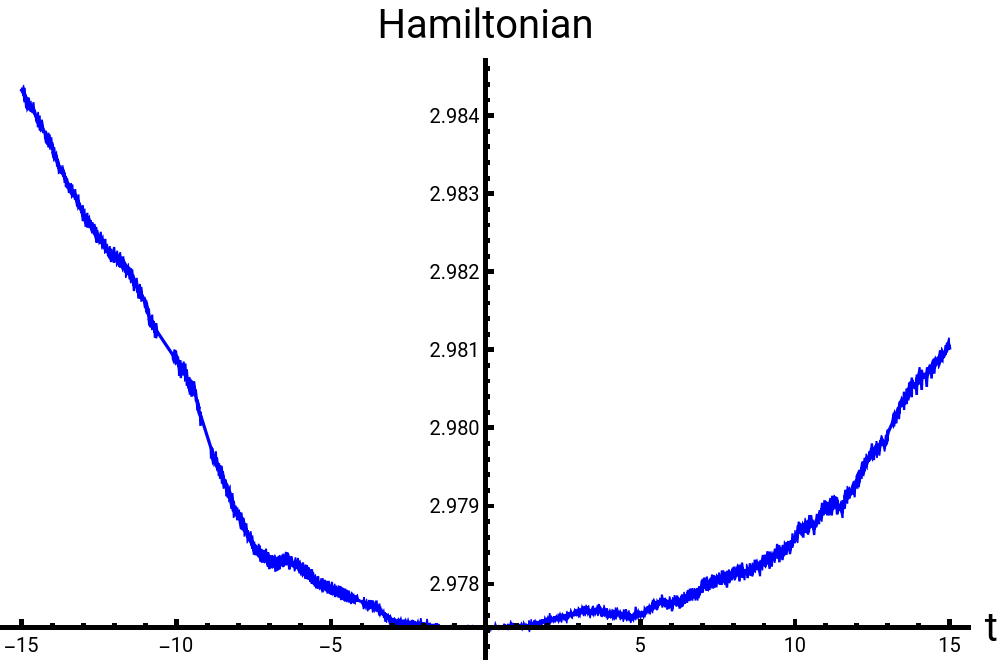
The complexity is used to define the non - equilibrium entropy and it can be shown that this entropy increases with complexity - this piece of code demonstrates that for our form of the pair inertia function . Complexity against time has a curve with a single minimum - this minimum is called the Janus point - and on both sides of that, the complexity increases . Hence, the entropy has a similar curve, and as increase in entropy is used to define the direction of the dynamical arrow of time, we get a dynamical arrow of time that points away from the Janus point .
TT=15;Qin1=RandomReal[{-0.5,0.5},{n}];Pin1=RandomReal[{-1,1},{n}];
For positive time
Firstpplot=Plot[Evaluate[Table[{p[i][s]}/.sol[eta,Qin1,Pin1,n,TT],{i,n}]],{s,0,TT},PlotRange->All,AxesLabel->{"t","Momenta"},PlotStyle->Directive[Thickness[0.005]]];Firstxplot=Plot[Evaluate[Table[{q[i][s]}/.sol[eta,Qin1,Pin1,n,TT],{i,n}]],{s,0,TT},PlotRange->All,AxesLabel->{"t","Positions"},PlotStyle->Directive[Thickness[0.005]]];FirstHplot=Plot[Evaluate[hamiltonian[Table[p[i][s],{i,n}],Table[q[i][s],{i,n}],eta]/.sol[eta,Qin1,Pin1,n,TT]],{s,0,TT},PlotRange->All,AxesLabel->{"Time","Hamiltonian"},PlotStyle->Directive[Blue]];Firstdiffsqplot=Plot[Evaluate[sumdiffsq[Table[p[i][s],{i,n}]]/.sol[eta,Qin1,Pin1,n,TT]],{s,0,TT},PlotRange->All,AxesLabel->{"t","P"},PlotStyle->Directive[Thickness[0.005],Blue]];
For negative time
TT=-TT;Secondpplot=Plot[Evaluate[Table[{p[i][s]}/.sol[eta,Qin1,Pin1,n,TT],{i,n}],{s,0,TT}],PlotRange->All,AxesLabel->{"t","Momenta"},PlotStyle->Directive[Thickness[0.005]]];Secondxplot=Plot[Evaluate[Table[{q[i][s]}/.sol[eta,Qin1,Pin1,n,TT],{i,n}],{s,0,TT}],PlotRange->All,AxesLabel->{"t","Positions"},PlotStyle->Directive[Thickness[0.005]]];SecondHplot=Plot[Evaluate[hamiltonian[Table[p[i][s],{i,n}],Table[q[i][s],{i,n}],eta]/.sol[eta,Qin1,Pin1,n,TT]],{s,0,TT},PlotRange->All,AxesLabel->{"Time","Hamiltonian"},PlotStyle->Directive[Blue]];Seconddiffsqplot=Plot[Evaluate[sumdiffsq[Table[p[i][s],{i,n}]]/.sol[eta,Qin1,Pin1,n,TT]],{s,0,TT},PlotRange->All,AxesLabel->{"t","P"},PlotStyle->Directive[Thickness[0.005],Blue]];TT=-TT;labelFontSize=20;(*Adjustthisforlargerlabels*)tickFontSize=10;(*Adjustthisfortickmarks*)
Generate Combined Hamiltonian Plot
combinedhamiltonianPlot=Show[FirstHplot,SecondHplot,PlotRange->All,ImageSize->500,(*8.6cmat300DPI*)AxesLabel->{Style["t",FontSize->labelFontSize],Style["Hamiltonian",FontSize->labelFontSize]},TicksStyle->Directive[FontSize->tickFontSize,Black],PlotStyle->Directive[Thickness[0.1]],AxesStyle->Directive[Thickness[0.005],Black]]
Out[]=
Generate combined position plot
Generate Combined Momentum Plot
Generate Combined Complexity Plot
Trajectory of four fractons in reduced space
Trajectory of four fractons in reduced space
For a system of n fractons, we always have that they split into more than one “Machian cluster”, where a Machian cluster is a set of fractons for which each pair in the cluster has a sizeable pair inertia function average at later times . For a system of 4 fractons, this means that our system spits into three non - trivial configurations - 3 - 1, 2 - 2 and 1 - 2 - 1, where our nomenclature is such that 1 - 2 - 1 means there are three clusters - one of two fractons and two of one fracton .
Fracton dynamics do not depend on the centre of mass position and momentum, so it is possible to use n - 1 “reduced” position and momentum coordinates, which obey the usual Poisson brackets and then the Hamiltonian only depends on these 2 (n - 1) coordinates . We now transform the 4 fracton problem from our typical x and p coordinates to these “reduced” coordinates .
Plot the solutions
Transform for positions and momenta to reduced coordinates
Defining the function for the specific case of four fractons in reduced coordinates
Hamiltonian function in reduced coordinates
Hamilton’ s equations of motion
Solve the equations
Plotting the reduced positions and momenta over time - for the positions and momenta we initially started with
For the four fracton problem, we have 3 reduced position and 3 reduced momentum coordinates .
Visualising the trajectory in the 3 D reduced position space
Visualising the trajectory in the 3 D reduced position space
If the fractons split into a cluster of 3 and a cluster of 1, the trajectory is like a billiard in an equilateral triangle (at late times) . If they split into 2 clusters of 2, we have the same thing in a square (at late times) . For 3 clusters, the trajectory is simply a billiard in a bound 1 D domain (at late times) .
CITE THIS NOTEBOOK
CITE THIS NOTEBOOK
Classical Fractons: local chaos, global broken ergodicity and an arrow of time
by Aryaman Babbar, Ylias Sadki, Abhishodh Prakash & S. L. Sondhi
Wolfram Community, STAFF PICKS, March 18, 2025
https://community.wolfram.com/groups/-/m/t/3419143
by Aryaman Babbar, Ylias Sadki, Abhishodh Prakash & S. L. Sondhi
Wolfram Community, STAFF PICKS, March 18, 2025
https://community.wolfram.com/groups/-/m/t/3419143