The ternary diagram presents the liquid-liquid equilibrium (LLE) behavior of the Methylcyclopentane/Hexane/Aniline system, with phase stability evaluated using the Tangent Plane Distance criterion (TPD_min). The sign of TPD_min serves as a thermodynamic indicator: compositions where TPD_min < 0 (cyan dots) are deemed unstable or metastable, as the system can lower its Gibbs energy by splitting into two coexisting liquid phases. These points cluster in the aniline-rich region of the diagram, reflecting aniline’s well-known limited miscibility with aliphatic hydrocarbons such as hexane and methylcyclopentane. Conversely, compositions where TPD_min > 0 (red dots) represent thermodynamically stable, single-phase mixtures, concentrated in the hydrocarbon-rich region where full miscibility is expected.
LLE diagram using the method based on common tangent plane and arc-length continuation
ClearAll["Global`*"];
universal gas constant
R=1.9872041;
temperature
T=273.15+45;
NRTL PARAMETERS
param={a13->0.3,a12->0.20,a32->0.30,B12->857.3718000,B21->2650.684300,B13->1410.932300,B31->2291.817900,B23->190.1605000,B32->-153.9573000,A12->-1.969300000,A13->-2.802700000,A23->0.0,A21->-7.132100000,A31->-5.248600000,A32->0.0};t13=A13+B13/T;t23=A23+B23/T;t12=A12+B12/T;t32=A32+B32/T;t31=A31+B31/T;t21=A21+B21/T;α={{0.,a12,a13},{a12,0.,a32},{a13,a32,0.}}/.param;τ={{0.,t12,t13},{t21,0.,t23},{t31,t32,0.}}/.param;
In[]:=
α//MatrixForm
Out[]//MatrixForm=
0. | 0.2 | 0.3 |
0.2 | 0. | 0.3 |
0.3 | 0.3 | 0. |
In[]:=
τ//MatrixForm
Out[]//MatrixForm=
0. | 0.725567 | 1.6321 |
1.19946 | 0. | 0.597707 |
1.95498 | -0.483914 | 0. |
G[i_,j_]:=Exp[-α[[i,j]]τ[[i,j]]];(*COMPOSITIONVECTOR*)xvec[x1_,x2_]:={x1,x2,1-x1-x2};(*NRTLACTIVITYCOEFFICIENTS*)lnGamma[i_,x1_,x2_]:=Module[{x,term1,term2},x=xvec[x1,x2];term1=Sum[x[[j]]τ[[j,i]]G[j,i],{j,1,3}]/Sum[x[[k]]G[k,i],{k,1,3}];term2=Sum[x[[j]]G[i,j]/Sum[x[[k]]G[k,j],{k,1,3}](τ[[i,j]]-Sum[x[[m]]τ[[m,j]]G[m,j],{m,1,3}]/Sum[x[[m]]G[m,j],{m,1,3}]),{j,1,3}];term1+term2];gamma[i_,x1_,x2_]:=Exp[lnGamma[i,x1,x2]];(*DIMENSIONLESSGIBBSENERGYOFMIXING:g/RT*)gmix[x1_,x2_]:=Module[{x},x=xvec[x1,x2];Sum[x[[i]]Log[x[[i]]],{i,1,3}]+Sum[x[[i]]lnGamma[i,x1,x2],{i,1,3}]];(*DERIVATIVES*)dgdx1[x1_,x2_]:=Evaluate[D[gmix[u,v],u]/.{u->x1,v->x2}];dgdx2[x1_,x2_]:=Evaluate[D[gmix[u,v],v]/.{u->x1,v->x2}];(*UNKNOWNS*)vars={x1a,x2a,x1b,x2b,m1,m2};(*COMMONTANGENTEQUATIONS*)eq1=dgdx1[x1a,x2a]==m1;eq2=dgdx1[x1b,x2b]==m1;eq3=dgdx2[x1a,x2a]==m2;eq4=dgdx2[x1b,x2b]==m2;eq5=gmix[x1b,x2b]-gmix[x1a,x2a]==m1(x1b-x1a)+m2(x2b-x2a);
EXTRA CONSTRAINT - Prevent trivial solution xα=xβ
eq6=(x1b-x1a)^2+(x2b-x2a)^2==d;
first value for d --- very small d=0.001 yield approximately the plait point
d0t=0.001;
solution
solct=FindRoot[{eq1,eq2,eq3,eq4,eq5,eq6/.d->d0t},{{x1a,0.1},{x2a,0.20},{x1b,0.70},{x2b,0.2},{m1,0.45},{m2,0.5}},MaxIterations->1000]
Out[]=
{x1a0.43817,x2a0.405496,x1b0.465024,x2b0.388797,m10.924659,m20.533594}
In[]:=
init={x1a[0]==(x1a/.solct),x2a[0]==(x2a/.solct),x1b[0]==(x1b/.solct),x2b[0]==(x2b/.solct),m1[0]==(m1/.solct),m2[0]==(m2/.solct),d[0]==d0t}
Out[]=
{x1a[0]0.43817,x2a[0]0.405496,x1b[0]0.465024,x2b[0]0.388797,m1[0]0.924659,m2[0]0.533594,d[0]0.001}
In[]:=
initdev={x1a'[0]==0.01,x2a'[0]==0.01,x1b'[0]==0.01,x2b'[0]==0.01,m1'[0]==0.01,m2'[0]==0.01,d'[0]==0.01}
Out[]=
{[0]0.01,[0]0.01,[0]0.01,[0]0.01,[0]0.01,[0]0.01,[0]0.01}
′
x1a
′
x2a
′
x1b
′
x2b
′
m1
′
m2
′
d
In[]:=
SYS={eq1,eq2,eq3,eq4,eq5,eq6}/.x1a->x1a[s]/.x1b->x1b[s]/.x2a->x2a[s]/.x2b->x2b[s]/.m1->m1[s]/.m2->m2[s]/.d->d[s];
In[]:=
Length@init
Out[]=
7
In[]:=
Length@initdev
Out[]=
7
In[]:=
Length[SYS]
Out[]=
6
In[]:=
auxeq=x1a'[s]^2+x1b'[s]^2+x2a'[s]^2+x2b'[s]^2+m1'[s]^2+m2'[s]^2+d'[s]^2==1
Out[]=
2
′
d
2
′
m1
2
′
m2
2
′
x1a
2
′
x1b
2
′
x2a
2
′
x2b
In[]:=
SYSFinal=Join[SYS,{auxeq},init,initdev];
In[]:=
Length@SYSFinal
Out[]=
21
In[]:=
SOL=NDSolve[SYSFinal,{x1a,x2a,x1b,x2b,m1,m2,d},{s,-100,100}]
Out[]=
x1aInterpolatingFunction,x2aInterpolatingFunction,x1bInterpolatingFunction,x2bInterpolatingFunction,m1InterpolatingFunction,m2InterpolatingFunction,dInterpolatingFunction


In[]:=
DATA1=Table[{x1a[s],x2a[s],1-x1a[s]-x2a[s]}/.SOL,{s,-17.7,0.020,0.01}];DATA2=Table[{x1b[s],x2b[s],1-x1b[s]-x2b[s]}/.SOL,{s,-17.7,0.020,0.01}];
In[]:=
Pt={{2,1},{0,Sqrt[3.]}}/2;
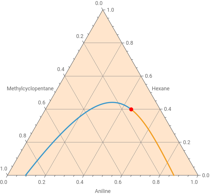
Type I liquid-liquid equilibrium (LLE) diagram - Plait point indicated in red
In[]:=
p0=Show[TernaryListPlot[{Flatten[DATA1,1],Flatten[DATA2,1]},Joined->True,PlotStyle->Thick,GridLines->Automatic,FrameLabel->{"Aniline","Hexane","Methylcyclopentane"},PlotRange->All,Method->{"Backdrop"->LightOrange}],Graphics[{Red,PointSize[0.02],Point[Pt.{x1a[s],x2a[s]}/.SOL/.s->0.020]}]]
Out[]=
TANGENT PLANE DISTANCE (TPD) ANALYSIS - case 1 : Liquid-liquid phase split expected
TANGENT PLANE DISTANCE (TPD) ANALYSIS FOR TERNARY LLE
FEED COMPOSITION
z={0.30,0.20,0.50};
NRTL ACTIVITY COEFFICIENTS
FEED ACTIVITY COEFFICIENTS
TPD FUNCTION
GLOBAL MINIMUM OF TPD
RESULTS
TANGENT PLANE DISTANCE (TPD) ANALYSIS - case 2 : Single liquid phase
TANGENT PLANE DISTANCE (TPD) ANALYSIS FOR TERNARY LLE
FEED COMPOSITION
FEED ACTIVITY COEFFICIENTS
TANGENT PLANE DISTANCE (TPD) ANALYSIS - case 3 : 100 randomly selected feed compositions
TANGENT PLANE DISTANCE (TPD) ANALYSIS yields expected results with red dots (single-phase region and positive TPD minimum) and cyan dots (two-phase region and negative TPD minimum)
CITE THIS NOTEBOOK
CITE THIS NOTEBOOK
Stability analysis of a ternary system using the tangent plane distance criterion
by Housam Binous
Wolfram Community, STAFF PICKS, June 7, 2026
https://community.wolfram.com/groups/-/m/t/3728973
by Housam Binous
Wolfram Community, STAFF PICKS, June 7, 2026
https://community.wolfram.com/groups/-/m/t/3728973