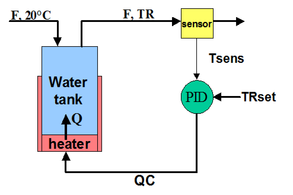
This problem is solved using Berkeley-Madonna in Ref. [1].
The solution using Mathematica is given in the present notebook. We would like to heat water with a heater. Outlet temperature must be equal to TRset=80°C. Inlet water temperature is equal to T0=20°C. Water flow is equal to F=10 m3/hr. Tank volume is equal to V=100 m3. Water density and heat capacity are rho=1 Kg/m3 and cp=4.19 KJ/(Kg °C). The heater and the temperature measurement device have a first order delay with a time constant equal to respectively TauQ and TauSens. Initial heat input and tank temperature are equal to 2500 KJ/hr and 20°C.
The solution using Mathematica is given in the present notebook. We would like to heat water with a heater. Outlet temperature must be equal to TRset=80°C. Inlet water temperature is equal to T0=20°C. Water flow is equal to F=10 m3/hr. Tank volume is equal to V=100 m3. Water density and heat capacity are rho=1 Kg/m3 and cp=4.19 KJ/(Kg °C). The heater and the temperature measurement device have a first order delay with a time constant equal to respectively TauQ and TauSens. Initial heat input and tank temperature are equal to 2500 KJ/hr and 20°C.
Proportional control. Kp is the proportional control constant.
In[]:=
V=100;F=10;rho=1;cp=4.19;Q0=2500;TRset=80;T0=20;TauSens=2;Kp=300;TauQ=1;
In[]:=
QC[t_]=Max[0,Q0+Kp (TRset-Tsens[t])]
Out[]=
Max[0,2500+300(80-Tsens[t])]
In[]:=
sol1=NDSolve[{V rho cp D[TR[t],{t,1}] F rho cp (T0-TR[t])+Q[t],
D[Q[t],{t,1}] (QC[t]-Q[t])/TauQ,
D[Tsens[t],{t,1}] (TR[t]-Tsens[t])/TauSens,TR[0] 20,
Tsens[0] 20,Q[0] 2500},{Q[t],Tsens[t],TR[t]},{t,0,150}]
D[Q[t],{t,1}] (QC[t]-Q[t])/TauQ,
D[Tsens[t],{t,1}] (TR[t]-Tsens[t])/TauSens,TR[0] 20,
Tsens[0] 20,Q[0] 2500},{Q[t],Tsens[t],TR[t]},{t,0,150}]
Out[]=
Q[t]InterpolatingFunction[t],Tsens[t]InterpolatingFunction[t],TR[t]InterpolatingFunction[t]


There is a delay between the tank temperature and the measured temperature. This is due to the sensor first order lag (TauSens=2).
In[]:=
plt1=Plot[{Evaluate[Tsens[t]]/.sol1,Evaluate[TR[t]]/.sol1},{t,0,60},PlotStyle{{Darker@Blue,Thick},{Darker@Red,Thick}},PlotRangeAll,AspectRatio->1,
GridLines-> Automatic,Frame->True,FrameLabel->{Style["time",14],Style["Tsens and TR",14]},ImageSize->400{1,1}]
GridLines-> Automatic,Frame->True,FrameLabel->{Style["time",14],Style["Tsens and TR",14]},ImageSize->400{1,1}]
Out[]=
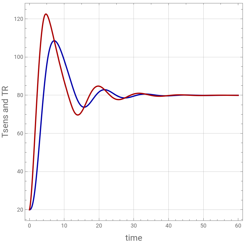
Tank temperature (TR=79.959) is slightly less than the set point = 80°C. It is common for proportional control to have a small offset error. Thus, we need to use a PI or a PID controller.
In[]:=
Evaluate[TR[t]]/.sol1/.t150
Out[]=
{79.9591}
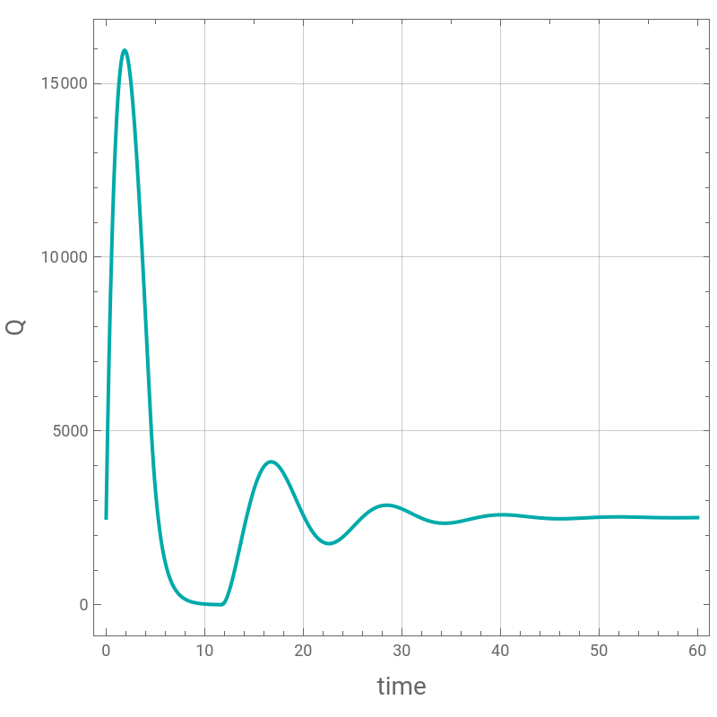
Heat input to water tank.
In[]:=
Plot[Evaluate[Q[t]]/.sol1,{t,0,60},PlotStyle{Darker@Cyan,Thick},PlotRangeAll,AspectRatio->1,
GridLines-> Automatic,Frame->True,FrameLabel->{Style["time",14],Style["Q",14]},ImageSize->400{1,1}]
GridLines-> Automatic,Frame->True,FrameLabel->{Style["time",14],Style["Q",14]},ImageSize->400{1,1}]
Out[]=
Proportional-Integral control. Kp and TauI are the proportional and the integral control constants.
In[]:=
V=100;F=10;rho=1;cp=4.19;Q0=2500;TRset=80;T0=20;TauSens=2;Kp=300;TauI=9;TauQ=1;
In[]:=
QC[t_]=Max[0,Q0+Kp (TRset-Tsens[t])+Kp/TauI Int[t]]
Out[]=
Max0,2500++300(80-Tsens[t])
100Int[t]
3
In[]:=
sol2=NDSolve[{V rho cp D[TR[t],{t,1}] F rho cp (T0-TR[t])+Q[t],
D[Q[t],{t,1}] (QC[t]-Q[t])/TauQ,
D[Tsens[t],{t,1}] (TR[t]-Tsens[t])/TauSens,
D[Int[t],{t,1}] TRset-Tsens[t],TR[0] 20,
Tsens[0] 20,Int[0] 0,Q[0] 2500},{Int[t],Q[t],
Tsens[t],TR[t]},{t,0,150}]
D[Q[t],{t,1}] (QC[t]-Q[t])/TauQ,
D[Tsens[t],{t,1}] (TR[t]-Tsens[t])/TauSens,
D[Int[t],{t,1}] TRset-Tsens[t],TR[0] 20,
Tsens[0] 20,Int[0] 0,Q[0] 2500},{Int[t],Q[t],
Tsens[t],TR[t]},{t,0,150}]
Out[]=
Int[t]InterpolatingFunction[t],Q[t]InterpolatingFunction[t],Tsens[t]InterpolatingFunction[t],TR[t]InterpolatingFunction[t]


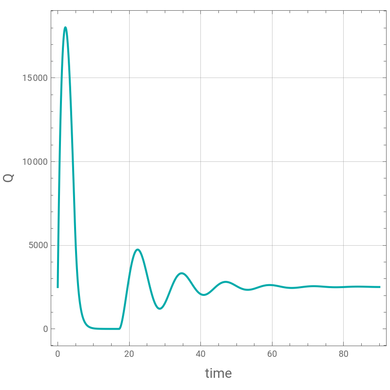
Tank temperature presents oscillatory behavior. Thus, we need to use a PID controller.
In[]:=
Plot[{Evaluate[Tsens[t]]/.sol2,Evaluate[TR[t]]/.sol2},{t,0,90},PlotStyle{{Darker@Blue,Thick},{Darker@Red,Thick}},PlotRangeAll,AspectRatio->1,
GridLines-> Automatic,Frame->True,FrameLabel->{Style["time",14],Style["Tsens and TR",14]},ImageSize->400{1,1}]
GridLines-> Automatic,Frame->True,FrameLabel->{Style["time",14],Style["Tsens and TR",14]},ImageSize->400{1,1}]
Out[]=
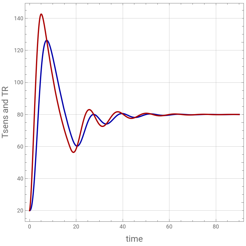
Tank temperature is exactly equal to the set point = 80°C.
In[]:=
Evaluate[TR[t]]/.sol2/.t150
Out[]=
{80.0003}
Heat input to water tank.
In[]:=
Plot[Evaluate[Q[t]]/.sol2,{t,0,90},PlotStyle{Darker@Cyan,Thick},PlotRangeAll,AspectRatio->1,
GridLines-> Automatic,Frame->True,FrameLabel->{Style["time",14],Style["Q",14]},ImageSize->400{1,1}]
GridLines-> Automatic,Frame->True,FrameLabel->{Style["time",14],Style["Q",14]},ImageSize->400{1,1}]
Out[]=
Proportional-Integral-Derivative control. Kp, TauI and TauD are the proportional, the integral and the differential control constants.
In[]:=
QC[t_]:=Max[0,
Q0+Kp (TRset-Tsens[t])+Kp/TauI Int[t]+Kp TauD D[ (TRset-Tsens[t]),{t,1}]]
Q0+Kp (TRset-Tsens[t])+Kp/TauI Int[t]+Kp TauD D[ (TRset-Tsens[t]),{t,1}]]
In[]:=
sol3=NDSolve[{V rho cp D[TR[t],{t,1}] F rho cp (T0-TR[t])+Q[t],
D[Q[t],{t,1}] (QC[t]-Q[t])/TauQ,
D[Tsens[t],{t,1}] (TR[t]-Tsens[t])/TauSens,
D[Int[t],{t,1}] TRset-Tsens[t],TR[0] 20,
Tsens[0] 20,Int[0] 0,Q[0] 2500},{Int[t],Q[t],
Tsens[t],TR[t]},{t,0,150}]
D[Q[t],{t,1}] (QC[t]-Q[t])/TauQ,
D[Tsens[t],{t,1}] (TR[t]-Tsens[t])/TauSens,
D[Int[t],{t,1}] TRset-Tsens[t],TR[0] 20,
Tsens[0] 20,Int[0] 0,Q[0] 2500},{Int[t],Q[t],
Tsens[t],TR[t]},{t,0,150}]
With a PID controller, temperature oscillations are quickly damped.
In[]:=
Plot[{Evaluate[Tsens[t]]/.sol3,Evaluate[TR[t]]/.sol3},{t,0,90},PlotStyle{{Darker@Blue,Thick},{Darker@Red,Thick}},
PlotRangeAll,AspectRatio->1, GridLines-> Automatic,Frame->True,FrameLabel->{Style["time",14],Style["Tsens and TR",14]},ImageSize->400{1,1}]
PlotRangeAll,AspectRatio->1, GridLines-> Automatic,Frame->True,FrameLabel->{Style["time",14],Style["Tsens and TR",14]},ImageSize->400{1,1}]
Difference between set point and actual tank temperature.
In[]:=
Plot[Evaluate[TRset-TR[t]]/.sol3,{t,0,70},
PlotStyle{Darker@Cyan,Thick},PlotRangeAll,AspectRatio->1,
GridLines-> Automatic,Frame->True,FrameLabel->{Style["time",14],Style["ΔT",14]},ImageSize->400{1,1}]
PlotStyle{Darker@Cyan,Thick},PlotRangeAll,AspectRatio->1,
GridLines-> Automatic,Frame->True,FrameLabel->{Style["time",14],Style["ΔT",14]},ImageSize->400{1,1}]
Heat input to water tank.
In[]:=
Plot[Evaluate[Q[t]]/.sol3,{t,0,70},PlotStyle{Darker@Cyan,Thick},PlotRangeAll,AspectRatio->1,
GridLines-> Automatic,Frame->True,FrameLabel->{Style["time",14],Style["Q",14]},ImageSize->400{1,1}]
GridLines-> Automatic,Frame->True,FrameLabel->{Style["time",14],Style["Q",14]},ImageSize->400{1,1}]
Tank temperature is exactly equal to the set point = 80°C.
In[]:=
Evaluate[TR[t]]/.sol3/.t150
References
References
[1] John Ingham, Irving J. Dunn, Elmar Heinzle, Jiri E. Prenosil, Jonathan B. Snape, Chemical Engineering Dynamics: An Introduction to Modelling and Computer Simulation, 3rd ed., Berlin: Wiley-VCH, 2007, pp. 420-424.
CITE THIS NOTEBOOK
CITE THIS NOTEBOOK
Temperature control of a water tank
by Housam Binous and Ahmed Bellagi
Wolfram Community, STAFF PICKS, July 26, 2023
https://community.wolfram.com/groups/-/m/t/2977163
by Housam Binous and Ahmed Bellagi
Wolfram Community, STAFF PICKS, July 26, 2023
https://community.wolfram.com/groups/-/m/t/2977163