Abstract: Data collection by organizations often results in inaccuracies, necessitating data cleaning as a crucial but time-consuming component of analysis. This essay examines a method for optimizing data points with errors such that all data points differ by a factor of n. The primary objective of this investigation is to develop more efficient techniques for data analysis. One significant finding of this computational essay is that machine learning models exhibit the same trends regardless of whether they are multiplied by a factor. This essay utilizes this finding to propose a more straightforward method of analysis.
In[]:=
WordCloud[WikipediaData["Analysis"]]
Out[]=
Unemployment Data Processing
Unemployment Data Processing
Initially, the data will be organized to enhance its visibility and facilitate analysis. Subsequently, it will be divided into training and testing sets to enable the evaluation of the model’s performance.
The Data
The Data
data=Import["C:\\Users\\ali12\\Downloads\\Unemployment Rate Data.xls"];preprocessedData=data/.Null->"";Dataset[preprocessedData]
Out[]=
Train-Test Split
Train-Test Split
In[]:=
whole=preprocessedData;{trainer,tester}=ResourceFunction["TrainTestSplit"][(#1->#2)&@@#&/@Drop[#&@@whole,11],Shuffle->False];Take[Dataset[trainer],3]Take[Dataset[tester],3]
Out[]=
Out[]=
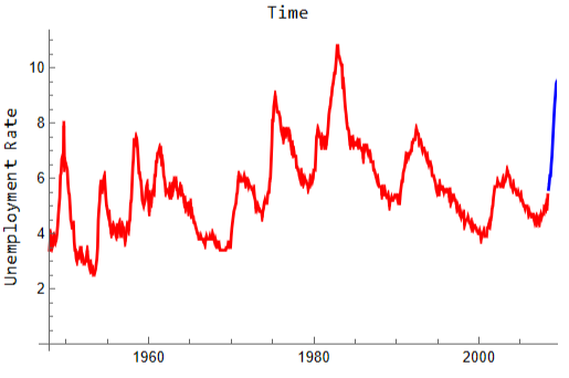
Data Visualisation: Train-Test Split
Data Visualisation: Train-Test Split
In[]:=
Labeled[Show[ListLinePlot[TimeSeries[trainer],PlotStyle->Red],ListLinePlot[TimeSeries[tester],PlotStyle->Blue]],{"Unemployment Rate","Time "},{Left,Top},RotateLabel->True]
Time Series Modeling
Time Series Modeling
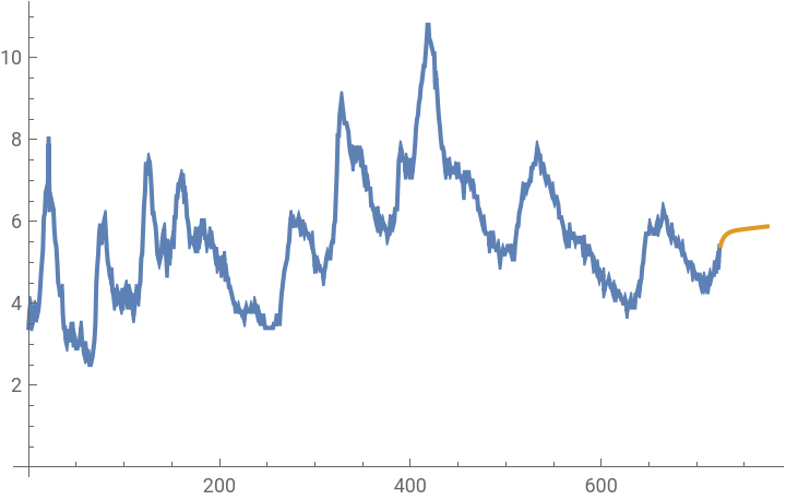
Typically, time series modeling is employed when working with time series data, as it tends to produce superior results on average. However, in this instance, machine learning techniques were utilized to evaluate their efficacy in comparison.
In[]:=
tsm=TimeSeriesModelFit[Values[trainer]]
Out[]=
TimeSeriesModel


In[]:=
Show[ListLinePlot[{tsm["TemporalData"],TimeSeriesForecast[tsm,{50}]}]]
Out[]=
Training Set by Applying a Factor of 2 to the Dataset
Training Set by Applying a Factor of 2 to the Dataset
The objective of this section is to provide a detailed examination of the processes involved in each stage, in order to enhance comprehension of the overall methodology. While the conventional approach for time series analysis involves the utilization of the TimeSeriesModelFit[] function, this essay will employ the machine learning function Predict[] for the purpose of model development.
Creating the Dataset
Creating the Dataset
In[]:=
multiplytwotrainer=Map[{#[[1]],#[[2]]*2}&,trainer];multiplytwotrainerWithRule=Rule@@@multiplytwotrainer;Take[Dataset[multiplytwotrainerWithRule],3]multiplytwotester=Map[{#[[1]],#[[2]]*2}&,tester];multiplytwotesterWithRule=Rule@@@multiplytwotester;Take[Dataset[multiplytwotesterWithRule],3]
Out[]=
Out[]=
Date Objects to Absolute Time
Date Objects to Absolute Time
In[]:=
multiplytwotrainerWithRuleinAbsolute=multiplytwotrainerWithRule/.Rule[x_,y_]:>Rule[AbsoluteTime[x],y];multiplytwotesterWithRuleinAbsolute=multiplytwotesterWithRule/.Rule[x_,y_]:>Rule[AbsoluteTime[x],y];Take[Dataset[multiplytwotrainerWithRuleinAbsolute],3]Take[Dataset[multiplytwotesterWithRuleinAbsolute],3]
The Machine Learning Model
The Machine Learning Model
Testing the Machine Learning Model
Testing the Machine Learning Model
Performance of the Machine Learning Model
Performance of the Machine Learning Model
Machine Learning Model Testing: Data Visualisation
Machine Learning Model Testing: Data Visualisation
The Machine Learning Model Error
The Machine Learning Model Error
The Error Equation
The Error Equation
It is anticipated that a similar approach will be employed to facilitate optimization in the subsequent section.
The Area Created by the Error
The Area Created by the Error
Training Set by Applying a Factor of n to the Dataset
Training Set by Applying a Factor of n to the Dataset
In this section, the objective is to analyze the patterns that persist across varying values of n, in order to demonstrate that the differences in predictions are nominal. Please note that for the rapid development of multiple machine learning models, it is recommended to utilize the Map function, as demonstrated in line 58, or to employ cloud functions and deployment capabilities available in Mathematica.
List of n
List of n
Function to generate training set with each data point adjusted by a factor of 2
Function to generate training set with each data point adjusted by a factor of 2
Machine Learning Models with a training set adjusted by a factor of n
Machine Learning Models with a training set adjusted by a factor of n
n and the corresponding predictors
n and the corresponding predictors
Function to test predictors
Function to test predictors
Testing the predictors
Testing the predictors
Processing Data for Visualization
Processing Data for Visualization
Visualize the Predictors Testing Results
Visualize the Predictors Testing Results
Proposal for a Method to analyse data
Proposal for a Method to analyse data
◼
Gather Data
◼
Determine a factor of n such that the actual data point y-value is equal to the x-value multiplied by n.
◼
The second bullet point should be optimized to minimize the error while attempting to determine the optimal value of n. The optimal value of n is defined as the value that transforms the data into a form that is easily analyzable, resembling an analytic function such as a polynomial, exponential function, trigonometric function, logarithm, or power function.
◼
Conduct an analysis of nominal trends and draw conclusions using a value of n equal to 1, incorporating new data into the analysis.
◼
In situations where the application of a particular method to the entire dataset is not beneficial, the dataset may be divided into smaller subsets, and the method may be applied to each subset individually.
Limitations
Limitations
◼
Best n value may differ based on optimisation technique
◼
Predict[] may not produce a 'good' machine learning model
◼
Only a few cases of n have been considered in this computation essay
Conclusion
Conclusion
In conclusion, the method proposed in this essay may offer a more efficient approach to data analysis and make machine learning more effective. However, it is important to note that its applicability has been demonstrated in a limited number of cases, as outlined in the limitations section. The ultimate goal of this investigation is to facilitate the development of more rapid analytical tools, enabling individuals and organizations to quickly identify trends and respond to changes in real-time. For instance, a government could use such tools to promptly address fluctuations in unemployment rates, thereby mitigating the negative consequences of delayed action. Stay tuned for my next project with the implemented method!
CITE THIS NOTEBOOK
CITE THIS NOTEBOOK
Uncovering unemployment trends: a machine learning approach to time series analysis
by Muhammad Ali Hafeez
Wolfram Community, STAFF PICKS, July 30, 2023
https://community.wolfram.com/groups/-/m/t/2979180
by Muhammad Ali Hafeez
Wolfram Community, STAFF PICKS, July 30, 2023
https://community.wolfram.com/groups/-/m/t/2979180