Liquid Liquid Equilibrium Curve and Tie Lines
for ternary system: hexane - heptane - methanol at 32.85 °C
Authors: Housam Binous and Ahmed Bellagi
Liquid Liquid Equilibrium Curve and Tie Lines
for ternary system: hexane - heptane - methanol at 32.85 °C
Authors: Housam Binous and Ahmed Bellagi
for ternary system: hexane - heptane - methanol at 32.85 °C
Authors: Housam Binous and Ahmed Bellagi
Reference: Housam Binous and Ahmed Bellagi, Calculation of Ternary Liquid - Liquid Equilibrium Data using Arc - Length Continuation, Engineering Reports, 3 (2), 2021.
Activities using the NRTL model
Gas constant, temperature and binary interaction parameters for the NRTL model
R=1.987;a13=0.42399900;a12=0.301800;a32=0.440800;t31=1287.78000;t13=1915.07700;t23=1598.3120000;t32=1566.43700;t12=-285.9411;t21=252.997600;T=273.15+32.85;
Computing Tie lines and LLE curve
Hexane = component 1
Heptane = component 2
Methanol = component 3
Hexane = component 1
Heptane = component 2
Methanol = component 3
In[]:=
K={GAMMA1/GAMMA1p,GAMMA2/GAMMA2p,GAMMA3/GAMMA3p}/.x31-x1-x2/.xp31-xp1-xp2;
In[]:=
z={0.5,0.1,0.4};sol=FindRoot(K[[i]]-1)z[[i]](1+(K[[i]]-1)ϕ)0,x1z[[1]](1+(K[[1]]-1)ϕ),x2z[[2]](1+(K[[2]]-1)ϕ),xp1K[[1]]z[[1]](1+(K[[1]]-1)ϕ),xp2K[[2]]z[[2]](1+(K[[2]]-1)ϕ),{ϕ,0.1,0.9},{x2,0.3,0.40},{x1,0.1,0.2},{xp1,0.6,0.7},{xp2,0.25,0.3},MaxIterations10000
3
∑
i=1
Out[]=
{ϕ0.358099,x20.0659509,x10.333336,xp10.798749,xp20.161034}
In[]:=
z={0.5,a,1-0.5-a}/.aa[s];
In[]:=
eq1=(K[[i]]-1)z[[i]]/(1+(K[[i]]-1)ϕ)0/.x1x1[s]/.x2x2[s]/.xp1xp1[s]/.xp2xp2[s]/.ϕϕ[s];eq2=x1z[[1]]/(1+(K[[1]]-1)ϕ)/.x1x1[s]/.x2x2[s]/.xp1xp1[s]/.xp2xp2[s]/.ϕϕ[s];eq3=x2z[[2]]/(1+(K[[2]]-1)ϕ)/.x1x1[s]/.x2x2[s]/.xp1xp1[s]/.xp2xp2[s]/.ϕϕ[s];eq4=xp1K[[1]]z[[1]]/(1+(K[[1]]-1)ϕ)/.x1x1[s]/.x2x2[s]/.xp1xp1[s]/.xp2xp2[s]/.ϕϕ[s];eq5=xp2K[[2]]z[[2]]/(1+(K[[2]]-1)ϕ)/.x1x1[s]/.x2x2[s]/.xp1xp1[s]/.xp2xp2[s]/.ϕϕ[s];eq6=x1'[s]^2+x2'[s]^2+xp1'[s]^2+xp2'[s]^2+ϕ'[s]^2+a'[s]^21;derivinit={x1'[0]0,x2'[0]0,xp1'[0]0,xp2'[0]0,ϕ'[0]1,a'[0]-0.2};init={x1[0](x1/.sol),x2[0](x2/.sol),xp1[0](xp1/.sol),xp2[0](xp2/.sol),ϕ[0](ϕ/.sol),a[0]0.05};
3
∑
i=1
In[]:=
system=Flatten[Join[{{eq1,eq2,eq3,eq4,eq5,eq6},derivinit,init}]];
In[]:=
SOL=NDSolve[system,{x1,x2,xp1,xp2,ϕ,a},{s,-1000,1000},AccuracyGoal5]

Out[]=
x1InterpolatingFunction,x2InterpolatingFunction,xp1InterpolatingFunction,xp2InterpolatingFunction,ϕInterpolatingFunction,aInterpolatingFunction


In[]:=
DATA1=Table[{x1[s],x2[s],1-x1[s]-x2[s]}/.SOL,{s,-7.650,1000,0.05}];
In[]:=
DATA2=Table[{xp1[s],xp2[s],1-xp1[s]-xp2[s]}/.SOL,{s,-7.650,1000,0.05}];
In[]:=
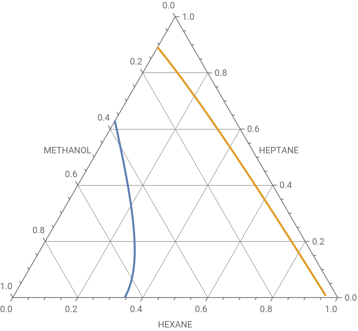
p1=TernaryListPlot[{Flatten[DATA1,1],Flatten[DATA2,1]},Joined->True,PlotStyle->Thick,GridLines->Automatic,FrameLabel->{"HEXANE","HEPTANE","METHANOL"}]
Out[]=
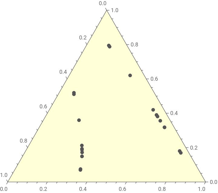
Tie Lines for Hexane-Heptane-Methanol Ternary System at 32.85°C obtained using LINGO.
In[]:=
dataLINGO={{0.3005868949109367,0.1488530639730277,0.5505600411160356},{0.6336205998460299,0.3177754567217978,0.04860394343217227},{0.2896143819212183,0.1720972620400208,0.5382883560387609},{0.5927000077642953,0.3563564394625065,0.0509435527731982},{0.2784778674318426,0.1930345981151117,0.5284875344530458},{0.5566976643962834,0.3901746388711372,0.05312769673257937},{0.2682339108928075,0.2124543772976846,0.519311711809508},{0.5247999187984354,0.4200681481909567,0.05513193301060782},{0.3004614037587242,0.1493299851602541,0.5502086110810217},{0.6328319138833067,0.3185228338234813,0.04864525229321195},{0.281450752522634,0.1873740909411266,0.5311751565362395},{0.5662380130405854,0.3812201247754143,0.05254186218400023},{0.1801587385264801,0.359577873923054,0.4602633875504659},{0.3081699225718108,0.6203719659911768,0.0714581114370124},{0.1132933315007217,0.7946614063365468,0.09204526216273144},{0.07463202508656841,0.5193554278628676,0.4060125470505641},{0.1208705345303362,0.7878058186934139,0.09132364677624988},{0.07891971135378113,0.51080919820414,0.410271090442079},{0.3320051659538572,0.06996757699681032,0.5980272570493326},{0.7898319690304335,0.1695368781253854,0.04063115284418115},{0.7786813318920752,0.1801603379532689,0.04115833015465582},{0.3301022128494239,0.07502233927581647,0.5948754478747597}};
In[]:=
Length[dataLINGO]
Out[]=
22
In[]:=
p2=TernaryListPlot[Table[{dataLINGO[[i]][[1]],dataLINGO[[i]][[2]],dataLINGO[[i]][[3]]},{i,1,22}],PlotStyle->{{Darker@Gray,PointSize[0.0175]},{Darker@Gray,PointSize[0.02]}},Method->{"Backdrop"LightYellow}]
Out[]=
In[]:=
Pt={{2,1},{0,Sqrt[3.]}}/2;
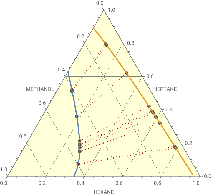
Plots of Liquid-Liquid Equilibrium Curve and Tie Lines for Hexane-Heptane-Methanol Ternary System at 32.85°C.
In[]:=
Show[p2,p1,Table[Graphics[{Dotted,Darker@Red,Line[{Pt.{dataLINGO[[i]][[1]],dataLINGO[[i]][[2]]},Pt.{dataLINGO[[i+1]][[1]],dataLINGO[[i+1]][[2]]}}]}],{i,1,22,2}]]
Out[]=