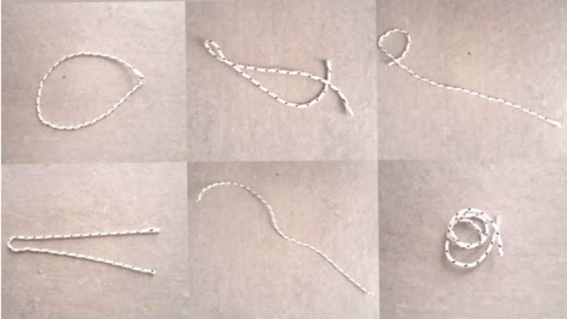
If a piece of rope is dropped on the floor, it can form multiple shapes, from ending up untangled and straight, to folding in half, to creating a spiral etc. These different outcomes dictate a variation in the distances between the two ends of the rope, every time it is dropped. Is it possible to find the distribution of these distances and the parameters that affect it?
Theoretical background
Theoretical background
As the rope is being dropped, gravitational and air drag forces are applied to each point of the rope. Since all the ropes we experiment with are uniform, the air drag force is applied equally to all points of the rope, as is gravity. Despite the gravitational force being applied to every point, not all of them react the same way due to the rope flexibility.
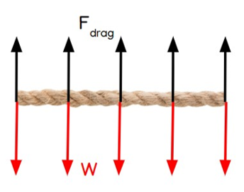
A piece of rope has multiple characteristics, but the ones that are important in this experiment are length, material, and thickness. When a rope is thicker, it has a higher modulus of elasticity (E).
Using Hooke’s law:
Using Hooke’s law:
σ = E*ε
where σ is the stress applied to a material, E is the modulus of elasticity and ε is the strain experienced by the material, we can explain why thicker ropes are harder to bend -require more stress for the same amount of strain-, and therefore will tend to create folds and spirals less often when dropped. Furthermore, we should consider the moment of inertia of the rope (assume rope to be a cylinder), where:
I=π*
1
4
4
r
The moment of inertia is proportional to the radius of the rope, so thicker ropes, with a bigger moment of inertia, will have greater resistance to bending. This means that for thicker ropes, we expect the distribution of distances to be shifted to the right, since the rope should land without bending, creating spirals or folding. Consequently, for thinner ropes we expect the distribution to be shifted to the left.
Experiment & Analysis
Experiment & Analysis
In this study, we will be using three 20cm pieces of rope from the same material, of varying thicknesses. The pre-drop placement and initial height was constant for every rope. Testing three rope pieces of different thickness, each rope was dropped 100 times and the distance between the two ends was measured. From these measurements we can obtain the distribution of distances for each rope.
Medium rope
Medium rope
For the medium rope, with a radius of r=5mm, the moment of inertia is:
In[]:=
i[r_]:=1/4*Pi*r^4;r=0.005;i[r]
Out[]=
4.90874×
-10
10
From the experiments, we get the following measurements:
In[]:=
alist={5.8,12.25,0.55,12,9.32,17.7,1,6.4,2.45,16,3.4,15.9,8,5,10.9,14,13,14,10.2,8.2,15,3.45,13,4.31,16.3,7.6,4.73,6.55,9,6.31,7,6.45,10.33,11.45,11.42,14,11.66,13.5,11,11.64,14.3,7.5,15.6,12.4,13.5,17.3,14.1,19.4,19.55,12,8.88,9,10,12.4,17,18.3,4.2,17.8,20,13.66,5.55,8.6,12.4,14.43,9.7,11.22,9.8,6.3,16.3,13.6,10.1,16.4,12,7.44,11.1,13.5,11,7.32,12.3,16.3,2,8,7.6,14.2,8,10.4,15.6,13,14.1,15,15.3,12.3,18.44,18.3,9.55,10,20,9.2,13.55,18.22}
In[]:=
Iconize[alist,"alist"]
Out[]=
In[]:=
Histogram[alist,20,ColorFunction->GrayLevel]
Out[]=
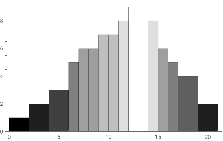
We can see that the distribution of distances resembles a normal distribution.
Thin rope
Thin rope
The thin rope has a radius of r=2.5mm, and its moment of inertia is:
In[]:=
r=0.0025;i[r]
Out[]=
3.06796×
-11
10
From the data obtained, we create the Histogram of the distribution of distances:
In[]:=
blist={5.8,2.25,0.55,12,0.32,7.7,2,6.4,2.45,16,3.4,5.9,8,5,0.9,4,3,4,10.2,8.2,5,13.45,0,1.31,6.3,7.6,4.73,6.55,9,6.31,7,6.45,10.33,1.45,12.42,14,2.66,13.5,11,11.64,4.3,7.5,5.6,1.4,0.8,7.3,4.1,5.4,5.5,2,8.88,0,10,2.4,18,6.3,3.2,17.8,2,3.66,5.55,2.6,1.4,4.43,0.7,1.22,9.8,6.3,4.3,3.6,10.1,2.4,1,7.44,11.1,3.5,3,7.32,4,1.3,4,8,6.6,4.2,8,2.4,3.6,3.25,4.1,15,5.3,2.3,1.44,8.3,9.55,1,3.2,9.2,3.55,4.22}
In[]:=
Iconize[blist,"blist"]
Out[]=
In[]:=
Histogram[blist,20,ColorFunction->GrayLevel]
Out[]=
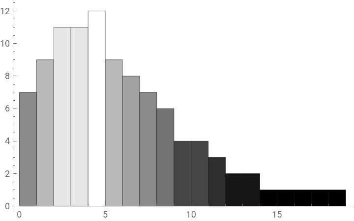
The distribution is indeed shifted to the left, because the rope is thinner, and therefore more prone to bending when dropped.
Thick rope
Thick rope
The thick rope’s radius is r=7.5mm and the moment of inertia is:
In[]:=
r=0.0075;i[r]
Out[]=
2.48505×
-9
10
The distribution of distances for this rope is the following:
In[]:=
clist={15.8,20,19.55,12,10.32,17.7,20,16.4,19.8,19,7.4,19.9,18,15,20,14,20,14,20,18.2,15,13.45,19,11.31,16.3,20,19.73,18,19,16.31,18,16.45,19.33,8.3,20,14,19.6,19,20,6.64,20,18.8,20,11.4,10.8,17.3,19.1,20,18.5,20,18,20,9,12.4,18,16.3,13.2,17.8,20,20,18.55,20,19.4,18.43,20,19.22,19.8,16.3,19.3,13.6,17.1,20,20,17.44,17.1,20,20,20,18.6,20,18.2,17.7,19,18.3,19,20,17.8,17.9,18.9,19,18,19,19,18.3,19.55,20,19.7,19.2,20,18.22}
In[]:=
Iconize[clist,"clist"]
Out[]=
Histogram[clist,20,ColorFunction->GrayLevel]
Out[]=
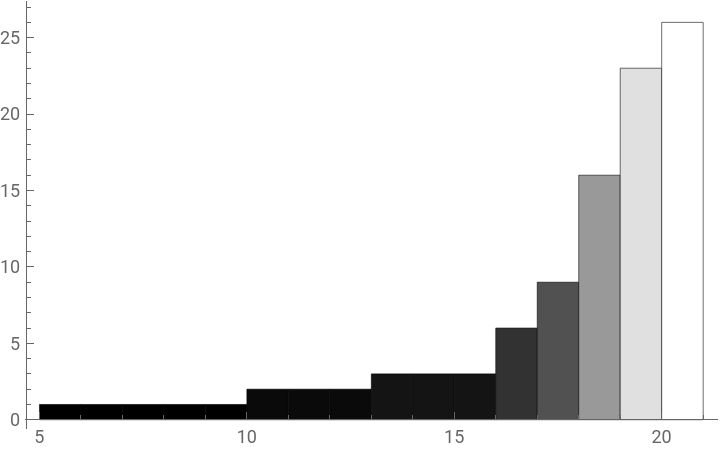
This distribution is shifted to the right, since the rope is thicker and has difficulty bending. It can also be noted that for this rope, there is no distance less than 5cm measured, which means that the rope’s resistance to bending prevents it from “folding” like the previous two.
Conclusion
Conclusion
Generally, when a piece of rope falls and the distances between the two ends are measured, the distribution of distances resembles a normal distribution. A rope’s tendency to fall in different ways is greatly dictated by its thickness. In thicker ropes, the distribution is shifted towards greater lengths, due to bending resistance, whereas in thinner ropes the distribution is shifted towards smaller distances, due to the ropes’ tendency to coil and fold when falling.
CITE THIS NOTEBOOK
CITE THIS NOTEBOOK
Distribution of distances between the two ends of a falling rope
by Myrto Terpsiadou
Wolfram Community, STAFF PICKS, April 23, 2024
https://community.wolfram.com/groups/-/m/t/3163238
by Myrto Terpsiadou
Wolfram Community, STAFF PICKS, April 23, 2024
https://community.wolfram.com/groups/-/m/t/3163238