This documents provide a quick and fast overview on different functionalities of the Wolfram quantum computation framework. For more info, please refer to our documentation pages.
Paclet installation
Paclet installation
The Wolfram Quantum Framework is a paclet. So first, let’s install it:
In[]:=
PacletInstall["https://wolfr.am/DevWQCF",ForceVersionInstall->True]<<Wolfram`QuantumFramework`
Out[]=
PacletObject

List of new quantum functions added:
In[]:=
Names["*Quantum*"]
Out[]=
{QuantumBasis,QuantumChannel,QuantumCircuitOperator,QuantumDistance,QuantumEntangledQ,QuantumEntanglementMonotone,QuantumMeasurement,QuantumMeasurementOperator,QuantumOperator,QuantumPartialTrace,QuantumPartialTranspose,QuantumState,QuantumTensorProduct,QuantumWignerTransform}
QuantumCircuitOperator
QuantumCircuitOperator
A quantum circuit is composition of quantum operators acting on a quantum state, representing a step-wise transformation of quantum system
a list of operators (either complete form, or shorthand)
QuantumCircuitOperator[{“named_circuit”,...}] a named-circuit
QuantumCircuitOperator[...][] a circuit acting on its corresponding register state
QuantumCircuitOperator[...][QuantumState[...]] a circuit acting on a quantum state
QuantumCircuitOperator[{op1,op1,op2}]
QuantumCircuitOperator[{“named_circuit”,...}] a named-circuit
QuantumCircuitOperator[...][] a circuit acting on its corresponding register state
QuantumCircuitOperator[...][QuantumState[...]] a circuit acting on a quantum state
Note in the following, we are showing the circuit diagram (QuantumCircuitOperator[...][“Diagram”]) which can be also obtained by applying TraditionalForm (or Command+Shift+T on Mac).
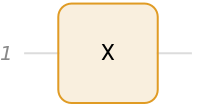
Pauli-X (by default on the qubit-1):
In[]:=
QuantumCircuitOperator["X"]
Out[]=
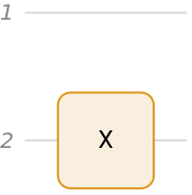
Pauli-X, acting on qubit-2:
In[]:=
QuantumCircuitOperator[{"X"->2}]
Out[]=
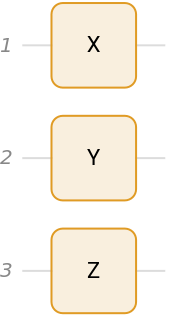
A Pauli string:
In[]:=
QuantumCircuitOperator["XYZ"]
Out[]=
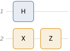
Pauli-X on qubit-2, Hadamard on qubit-1 (note, by default, it is always 1st one), and Pauli-Z on qubit-2:
In[]:=
QuantumCircuitOperator[{"X"->2,"H","Z"->2}]
Out[]=
CNOT (by default qubit-1 as control and qubit-2 as target)
In[]:=
QuantumCircuitOperator[{"CNOT"}]
Out[]=
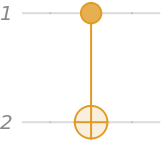
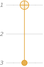
CNOT with qubit-3 as the control and qubit-1 as the target:
In[]:=
QuantumCircuitOperator[{"CNOT"->{3,1}}]
Out[]=
Note that a circuit is in fact a composition of operators (composition in usual sense, and also in Wolfram Language sense)
Once can extract the sequence of operators/gates using “Operators” as a property:
Once can extract the sequence of operators/gates using “Operators” as a property:
In[]:=
qc=QuantumCircuitOperator[{"X"->2,"H","Z"->2,1,{2}}]
Out[]=
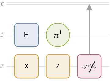
In[]:=
qc["Operators"]
Out[]=
QuantumOperator,QuantumOperator,QuantumOperator,QuantumOperator,QuantumMeasurementOperator


Additionally, an overall operator can be extracted too:
In[]:=
qc["CircuitOperator"]
Out[]=
QuantumMeasurementOperator

Overall, a circuit can contains many different transformations, here:
Hadamard on qubit-1, CNOT with qubit-1 as control and 2 as target, RootNOT/V on qubit-1, a barrier (for visualization purposes), RootSWAP on qubit-1 and 2, generic rotation Exp[-θ/2XY] on qubit 1 and 2, permutation on qubit 1 and 2, a barrier, a quantum channel (bit flip with probability p) on qubit-1, a barrier, and measurements (in computational basis) on qubits 1 and 2
Hadamard on qubit-1, CNOT with qubit-1 as control and 2 as target, RootNOT/V on qubit-1, a barrier (for visualization purposes), RootSWAP on qubit-1 and 2, generic rotation Exp[-θ/2XY] on qubit 1 and 2, permutation on qubit 1 and 2, a barrier, a quantum channel (bit flip with probability p) on qubit-1, a barrier, and measurements (in computational basis) on qubits 1 and 2
In[]:=
qc=QuantumCircuitOperator[{"H","CNOT",Sqrt@"X","Barrier",QuantumCircuitOperator["Fourier"],"RootSWAP",{"R",θ,"X"->1,"Y"->2},{"Permutation",Cycles[{{1,2}}]},"Barrier",QuantumChannel[{"BitFlip",p}],"Barrier",{1},{2}}]
Out[]=

There are lots of interesting visualization features. We refer out readers to our documentation on Diagram.
And list of operations/transformations on above circuit:
In[]:=
qc["Operators"]
Out[]=
QuantumOperator,QuantumOperator,QuantumOperator,QuantumCircuitOperator,QuantumOperator,QuantumOperator,QuantumOperator,QuantumChannel,QuantumMeasurementOperator,QuantumMeasurementOperator


QuantumOperator
QuantumOperator
The most important pattern to remember is QuantumOperator[arg,order]. Note by default, the order is set as {1}, or {1,2}, or {1,2,...} (depending on the operator)
Pauli-X operator, acting on qubit-1:
In[]:=
QuantumOperator["X"]
Out[]=
QuantumOperator

SWAP operator, acting on qubit-1 and 2:
In[]:=
QuantumOperator["SWAP"]
Out[]=
QuantumOperator

Permutation operator with a given cycle, acting on qubit-1, 2, and 3:
In[]:=
QuantumOperator[{"Permutation",Cycles[{{1,3,2}}]}]
Out[]=
QuantumOperator

SWAP operator, acting on qubit-2 and 3:
In case, to help with the order, you can always visualize operators in a circuit:
Some arithmetic/operations on operators:
Exponential of an operator (similar to time-evolution of a time-independent operator, or rotation operator):
Taking square-root of an operator:
which is the same as the named SX operator:
Creating a summation of two operators:
The same can be created by adding two operators (instead of using shorthand version above):
Another example on adding operators:
Testing that it is the same as creating operators separately and then adding them:
A generic Rotation operator Exp[- θ/2(XX+YY+ZZ)]:
Since each term in the exponent commutes with others, we can write above operator as multiplication of three operators:
One can define controlled-operators with many control and target
An operator is a tensor flow with input and output:
Named-circuits
Named-circuits
Bell circuit:
Toffoli gate (decomposed form):
quantum Fourier transform (by default two qubits):
quantum Fourier transform with 3-qubits:
quantum phase estimation, for QuantumOperator[{“Phase”,2π/5}], in four steps (ie using 4-qubits)
Bernstein-Vazirani circuit, given a secret string:
Graph circuit, given a graph:
Grover search algorithm, given a Boolean function:
Ising-type of interactions and their Trotter-Suzuki decomposition (4th order)
QuantumBasis
QuantumBasis
If not specified, we automatically treat everything in the computational basis.
Important patterns to remember:
QauntumBasis[{n1,n2,...}]
QuantumBasis[n,m]
QuantumBasis[asso]
Important patterns to remember:
QauntumBasis[{n1,n2,...}]
QuantumBasis[n,m]
QuantumBasis[asso]
3D basis:
2×3×5 dimensional basis:
A customized basis, with two vectors:
There are also many named basis:
QuantumState
QuantumState
The most important pattern to remember is QuantumBasis[arg,qb], with qb defining the basis (if not specified, will be treated automatically as computational basis, given dimensions of arg
arg: a list of amplitudes, or density matrix, or named-states
arg: a list of amplitudes, or density matrix, or named-states
A 2D quantum state given a state vector:
A 2D quantum state given a state vector:
named-states
Werner state:
Some arithmetic with states
Basis transformation: a state defined in the computational basis, then transformed into Pauli-X basis
there are couple of functions one can apply on quantum states
QuantumPartialTrace
QuantumDistance
QuantumEntangledQ
QuantumEntanglementMonotone
QuantumPartialTrace
QuantumDistance
QuantumEntangledQ
QuantumEntanglementMonotone
Create a Werner state in d=2, with a probability p (note, it is symbolic state, p is a symbol) and then trace out the 2nd system and return the formula:
For example, Werner states with p>=1/2 are not entangled, while p<1/2 are
Create a GHZ state and test if it is entangled or not:
Create a GHZ state, and test if the qubit-1 and qubit-2 are entangled in that state, or not:
Concurrence (default), EntanglementEntropy, LogNegativity, Negativity, {“RenyiEntropy”,α}, Realignment
Calculate the LogNegativity (as entanglement monotone metric) for a given Werner state:
There are lots of interesting properties one can get from a quantum state:
StateVector, DensityMatrix, Tensor, Norm, TraceNorm, Transpose, SchmidtBasis, Conjugate, Transpose (and partial transpose), Purify (and Unpurify), Bend (Unbend), Bipartition
StateVector, DensityMatrix, Tensor, Norm, TraceNorm, Transpose, SchmidtBasis, Conjugate, Transpose (and partial transpose), Purify (and Unpurify), Bend (Unbend), Bipartition
Note some of these properties return eg a numerical value (Entropy) and some returns a quantum state (Transpose, or Bipartition)
Generate a random pure state of 2-qubits:
Decompose it (iteration of Schmidt decomposition, until getting separable terms; ie no entanglement)
Similar operator, but final terms are still 2-qubit states (but separable)
Note partial tracing over ancillary qudit returns the original state
Permute:
Note an operation can be defined by states (|a><b| format of QM) or an operator (difference in our framework: input/output qudits)
Note quantum state is a tensor flow with no input and one or more output (depending on the number of qudits)
QuantumMeasurementOperator
QuantumMeasurementOperator
Either usual PVMs or generic POVMs
Think of it very similar to quantum operator (given basis, and order)
Think of it very similar to quantum operator (given basis, and order)
POVM:
CITE THIS NOTEBOOK
CITE THIS NOTEBOOK
Wolfram Quantum Framework: a fast introduction
by Mohammad Bahrami
Wolfram Community, STAFF PICKS, November 1, 2022
https://community.wolfram.com/groups/-/m/t/2679491
by Mohammad Bahrami
Wolfram Community, STAFF PICKS, November 1, 2022
https://community.wolfram.com/groups/-/m/t/2679491