Finite Abstract Simplicial Complexes
by Oliver Knill, Harvard University, 11/19/2020
by Oliver Knill, Harvard University, 11/19/2020
We illustrate some theorems which have been discovered first by playing around and experimenting using Mathematica before the results were proven theoretically. The topic deals with one of the simplest possible geometric structure which exists in mathematics, finite sets of sets which are closed under the operation of taking finite subsets. Despite the simplicity having only one axiom, the structure is incredibly rich.
Complexes
Complexes
A finite set of set which is closed under the operation of taking finite non-empty subsets is called a finite abstract simplicial complex. An arbitrary set of sets generates such a structure by closing it over all subset formations:
In[]:=
Generate[A_]:=Delete[Union[Sort[Flatten[Map[Subsets,A],1]]],1];G=Generate[{{1,2},{3,5},{2,6,8}}]
Out[]=
{{1},{2},{3},{5},{6},{8},{1,2},{2,6},{2,8},{3,5},{6,8},{2,6,8}}
In order to experiment, we want to generate random complexes. Here is an example to generate a random complex for which we take m sets in [n]={1,...,n}.
In[]:=
RandomSets[n_,m_]:=Module[{A={},X=Range[n],k},Do[k:=1+Random[Integer,n-1];A=Append[A,Union[RandomChoice[X,k]]],{m}];Sort[Generate[A]]];G=RandomSets[6,12]
Out[]=
{{1},{2},{3},{4},{5},{6},{1,2},{1,3},{1,4},{1,5},{1,6},{2,3},{2,4},{2,5},{2,6},{3,4},{3,5},{3,6},{4,5},{4,6},{5,6},{1,2,3},{1,2,4},{1,2,5},{1,2,6},{1,3,4},{1,3,5},{1,4,5},{1,4,6},{1,5,6},{2,3,6},{2,4,5},{2,4,6},{2,5,6},{3,4,5},{3,5,6},{4,5,6},{1,2,4,5},{1,2,4,6},{1,2,5,6},{1,3,4,5},{1,4,5,6},{2,4,5,6},{1,2,4,5,6}}
An example is the icosahedron complex made of 20 triangles. It realizes a triangulation of a two-dimensional sphere
In[]:=
icosahedron=Generate[{{1,2,5},{1,2,6},{1,3,4},{1,3,5},{1,4,6},{2,5,9},{2,6,10},{2,9,10},{3,4,8},{3,5,11},{3,8,11},{4,6,12},{4,8,12},{5,9,11},{6,10,12},{7,8,11},{7,8,12},{7,9,10},{7,9,11},{7,10,12}}];
The Euler characteristic of a complex super sums the sizes of the sets. The even dimensional sets (sets of odd length) are given weight 1, the odd dimensional sets (sets of even length) are given weight -1. For the Icosahedron just defined, the Euler characteristic is 2, as we know from the Euler formula
In[]:=
Omega[x_]:=-(-1)^Length[x];EulerChi[G_]:=Total[Map[Omega,G]];EulerChi[icosahedron]
Out[]=
2
Graphs
Graphs
We can visualize a complex by building finite simple graphs from it. There are two important graphs one can get from a complex G. The first is called the Barycentric refinement graph of G because its clique complex is the Barycentric refinement of the simplicial complex. The nodes of the graph are the sets. Two nodes are connected, if one is contained in the other.
In[]:=
BarycentricGraph[G_]:=Module[{n=Length[G],v,e,s},v=Range[n];e={};Do[If[(SubsetQ[G[[k]],G[[l]]]||SubsetQ[G[[l]],G[[k]]])&&Not[G[[k]]G[[l]]],e=Append[e,v[[k]]v[[l]]]],{k,n},{l,k+1,n}];s=UndirectedGraph[Graph[v,e]]];ConnectionGraph[G_]:=Module[{n,A},n=Length[G];A=Table[1,{n},{n}];Do[If[DisjointQ[G[[k]],G[[l]]]||G[[k]]G[[l]],A[[k,l]]=0],{k,n},{l,n}];AdjacencyGraph[A]];
In[]:=
G=icosahedron;GraphPlot3D[BarycentricGraph[G]]
Out[]=

In[]:=
GraphPlot3D[ConnectionGraph[G]]
Out[]=

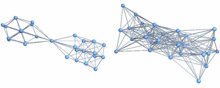
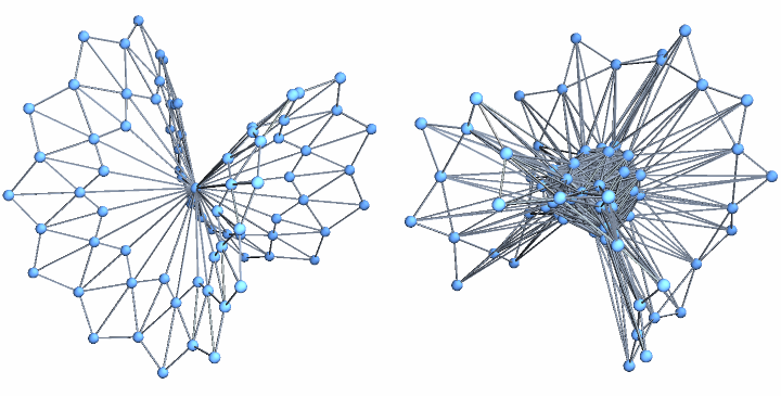
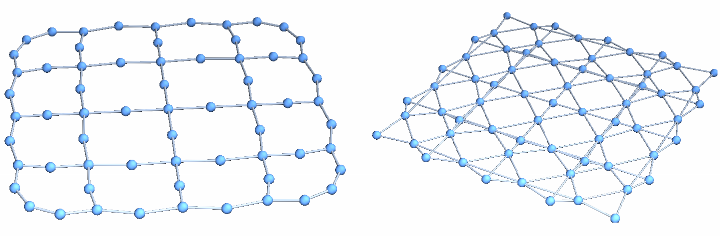
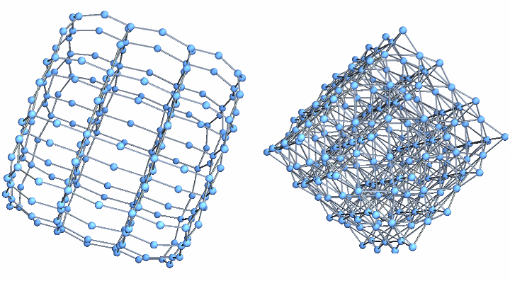
The connection matrix L as well as the connection graph contain all the information about the complex. One can reconstruct the sets from it. The connection graph looks a bit messy but it has the amazing property that the Fredholm Laplacian L = 1+L is always unimodular and therefore is invertible. Here are more examples:
In[]:=
G=Generate[Union[{Range[4]},{Range[4]+3}]];GraphicsGrid[{{GraphPlot3D[BarycentricGraph[G]],GraphPlot3D[ConnectionGraph[G]]}}]
Out[]=
In[]:=
G=Generate[FindClique[WheelGraph[20],Infinity,All]];GraphicsGrid[{{GraphPlot3D[BarycentricGraph[G]],GraphPlot3D[ConnectionGraph[G]]}}]
Out[]=
In[]:=
G=Generate[FindClique[GridGraph[{5,5}],Infinity,All]];GraphicsGrid[{{GraphPlot3D[BarycentricGraph[G]],GraphPlot3D[ConnectionGraph[G]]}}]
Out[]=
In[]:=
EulerChi[Generate[FindClique[ConnectionGraph[G]]]]
Out[]=
1
In[]:=
G=Generate[FindClique[GridGraph[{4,4,4}],Infinity,All]];GraphicsGrid[{{GraphPlot3D[BarycentricGraph[G]],GraphPlot3D[ConnectionGraph[G]]}}]
Out[]=
Refinement
Refinement
The Barycentric refinement of a complex is its order complex. According to Dieudonne, incidence matrices, duality, refinement are the three pillars in the foundation of combinatorial topology. Barycentric refinement has a lot of nice properties like that the topology does not change and that one gets closer and closer to the continuum. Doing refinements of a triangle is iconic.
In[]:=
Barycentric[G_]:=Generate[FindClique[BarycentricGraph[G],Infinity,All]];Barycentric[G_,n_]:=Last[NestList[Barycentric,G,n-1]];
Here is the third Barycentric refinement of the triangle:
In[]:=
G=Barycentric[Generate[{Range[3]}],3];GraphPlot3D[BarycentricGraph[G]]
Out[]=

Here is the second Barycentric refinement of the tetrahedron:
Here is the second Barycentric refinement of the icosahedron
The central limit theorem for Barycentric refinement tells that the eigenvalues of any Laplacian, like the Kirchoff Laplacian converges in the Barycentric limit weakly to a measure which only depends on the maximal size of a set in G. What we see here is the inverse of the integrated density of states. We see spectral gaps already if the maximal dimension of G is 2 or more. These spectra are universal in the sense that it does not matter with what complex we start as long as the maximal dimension is the same. Lets look at a simple example. Already after three refinements, the spectral curves look the same.
Connections
Connections
The connection matrix of the complex G is the identity matrix plus the adjacency matrix of the connection graph. It is the matrix with entries L(x,y) = 1 if x and y intersect and L(x,y)=0 if they don’t. The unimodularity theorem tells that that this matrix always has determinant 1 or -1. The inverse of the matrix is then an integer matrix too:
Since we think about L as a Laplacian, the entries of the inverse as Green functions. They are important in physics. We usually think of Green function entries g(x,y) as potential energies between two points. This works also here, but unlike for the usual Laplacians in physics where g(x,x) is undefined, we have now always finite values. The total potential energy is the sum over all pairs x,y. The energy theorem tells that this is the same than the Euler characteristic of G.
The number of positive eigenvalues of L minus the number of negative eigenvalues of L is also the Euler characteristic of G:
Cohomology
Cohomology
Besides connection relations, there are also incidence relations. One defines first the exterior derivative d, which consists of the discrete analogues of grad, curl or div, then forms the Dirac operator D=d+d*, then computes the Hodge Laplacian L=D^2. This operator has the various form Laplacians as blocks. The zero’th block for example is the Kirchhoff Laplacian. The kernel of the k’th block form a basis of the k’th cohomology group. We compute it here for the icosahedron complex. The code below allows to compute the cohomology for any complex
Both the Dirac operator D and the Hodge Laplacian H have the same size than the connection Laplacian. Lets look at them. In this case, because the complex is two dimensional, there are three cohomology groups. They are spanned by the k-harmonic forms. For example, a basis for the zero’th cohomology group are the locally constant functions. The first cohomology group is zero for simply connected complexes like the icosahedron. The second cohomology group then is the same as the zero’th. The Theorem of Euler-Poincare assures that the Euler characteristic of G is the same than the alternating sum of the Betti numbers. Indeed 1-0+1=2 is the Euler characteristic of the Icosahedron.
Many theorems from the continuum go over verbatim to the discrete. An example is the McKean-Singer formula telling that the Euler characteristic of G is equal to the super trace str(exp( -t H)) for the Hodge Laplacian. First of all, we need to find the size of the blocks and then break up H to get the list HH of blocks:
Here is the super trace of exp(-H). It agrees with the Euler characteristic. This works for any simplicial complex, not only for discrete manifolds. The reason is a simple super symmetry between even-dimensional and odd-dimensional discrete differential forms. The union of the non-zero eigenvalues of the even forms is the same than the union of the non-zero eigenvalues of the odd forms:
Here is a again an illustration of the general Euler-Poincare formula which assures that the super sum of the Betti numbers is the Euler characteristic. The Betti numbers are the dimensions of the null spaces of the blocks:
Energy
Energy
There is more to the connection calculus story. We can attach to every set in G a number f(x) and then define an energy of a subset A of G as the sum of the f values. This is a discrete integration and gives an analogue of the Euler characteristic. Now, given a set x, we can look at the star of x, which is the set of all sets containing x and the core of x, the set of all sets contained in x. Now we can define the matrix L(x,y) as the energy of the intersection of the star of x and y and the matrix g(x,y) as the energy of the intersection of the cores of x and y, conjugated by the checkerboard matrix S(x,y) which is 1 if x,y have both either even or odd dimension and S(x,y)=-1 if one of them has even and the other odd dimension. We started above with the special case where the energy function f(x) was (-1)^dim(x) in which case L(x,y)=1 if x,y intersect and L(x,y)=0 else. There are four theorem: Theorem 1 tells that the sum of all the g-values is the Euler characteristic. There is also a quadratic Ising type interaction energy. Theorem 2 allows to expressed it as the super-sum over all squares of the Green function entries. Theorem 3 assures that the determinant of L is equal to the determinant of g and is equal to the product of the energy values. Finally, Theorem 4 assures that if the energy values f(x) have length 1 everywhere, then L and the conjugate of g are inverse matrices. This happens for example for {-1,1} valued functions or then for complex unit circle valued functions. Here is the code which had been used to discover these relations. For convenience, we start from scratch. The following few lines are independent of all previous code. It should be pretty self-explanatory. One of the nice features of Mathematica is to be able to write short library independent code:
Deformation
Deformation
Given a complex G, it defines the exterior derivative d and so the Dirac operator D. By Connes formula, the Dirac operator allows to recover the metric on a Riemannian manifold. That is also true in the discrete. If we deform the operator D isospectrally, then this can be seen as a motion on a group of symmetries of the geometry. The amazing mathematical fact is that when doing the isospectral deformation, there is an expansion of space with an inflationary start. Also interesting is that the Dirac operator D develops a diagonal part. On a classical level, the deformation is invisible because the Hodge Laplacian does not change. However, the metric expands. Also the following part is
Here we see how the Dirac operator deforms. The side diagonal parts which were the only thing initially fade (distances expand).
The exterior derivative d has become small (space has expanded), but it still satisfies d^2=0, so that the cohomology does not change. The Dirac operator D has developed a diagonal block part. We still have D.D=H. The Hodge Laplacian does not change through the deformation. All physics which involves the Hodge Laplacian does not see the deformation.
References
References
[1] O. Knill, The energy of a simplicial complex, Linear Algebra and its Applications, 600, pages 96-129, 2020
[2] O. Knill, The amazing world of simplicial complexes, https://arxiv.org/abs/1804.08211, 2018
[3] O. Knill, Green functions of Energized complexes, https://arxiv.org/abs/2010.09152, 2020
[2] O. Knill, The amazing world of simplicial complexes, https://arxiv.org/abs/1804.08211, 2018
[3] O. Knill, Green functions of Energized complexes, https://arxiv.org/abs/2010.09152, 2020