This notebook series is designed to introduce selected dynamic economic models to both advanced undergraduate and graduate students. Economists have relied on a series of economic models to better understand the otherwise highly complex causal relationship among many economic variables. Dynamic economic models set up by systems of either difference or differential equations are particularly useful in tracing the change in the quantity of unknown economic variables (e.g., the capital stock, demand for labor, aggregate output, etc.) and their interactions over time.
This notebook series aims to help students better understand the depth, usefulness, and limitations of major existing micro and macroeconomic models by demonstrating how we can use Wolfram Mathematica to replicate and reconstruct the core ideas and find dynamic solution of the model.
The model introduced in this notebook series include, among others, (1) the cobweb model of the quantity and price adjustment, (2) Keynes’s aggregate demand model, (3) Hicks’s ISLM model, (4) Samuelson’s investment accelerator model, (5) Kalecki’s investment delay model, (6) the predator-prey interaction model, (7) the epidemic model, (8) Ricardo’s three dimensional business cycle model, (9) Marx-Goodwin business cycle and growth model, (10) Smith’s and Ricardo’s growth model, (11) the Harrod-Domar growth model, (12) the Solow growth model, (13) the RBC model, (14) Romer’s new growth model, and (15) the circuit of capital model.
A classical Marxian critique of Solow’s aggregate production function
Introduction
Introduction
As we saw in the previous notebook, Robert Solow introduced the technology-augmented aggregate production function in his growth model (Solow 1957). Since then, his function has been widely used in many theoretical and empirical studies in economics. One particular mathematical function that has the same constant returns to scale (CRS) property is the Cobb-Douglas function. Thanks to this convenient property, this function has been used in many economic modeling exercises, both in macro and microeconomic fields, to represent the aggregate production function. In the previous session, we learned that the Cobb-Douglas functional specification of the aggregate production function enabled us to (1) derive the intensive form of the production model easily and (2) compute and visualize the solution curves, i.e., aggregate output per effective worker and investment per effective worker quickly.
But there is one fundamental problem in this conventional practice. In Solow’s model, the exact meaning of the A term and the two exponents appearing in the Cobb-Douglas function is not properly explained. What does the A term mean? Do these two exponents represent the intensity and/or productivity of both capital and labor inputs? Do these exponents also imply proportional ‘factor rewards,’ resulting in an equitable distribution of national income along the line of marginal productivity principle?
According to one famous classical Marxian economist Anwar Shaikh (Shaikh 1974), the Cobb-Douglas form of Solow’s aggregate production function is merely an algebraic derivation result from the national income account identity, rather than revealing some fundamental laws of economics that explain the real-world production and income distribution activity (See also Shaikh 1980; 1987; 2005 and Felipe and McCombie 2006; 2012). Shaikh shows that the A term and two exponents used in the Cobb-Douglas functional specification of the aggregate production function implicitly assumes the constancy of income distribution between capital and labor input. If there is no such a constant income share assumption, however, we cannot even use this function as a representation of how the economy works.
This notebook reconstructs Shaikh’s critique of the Cobb-Douglas form of the aggregate production function used in Solow’s technology-augmented growth model. A step-by-step derivation of crucial equations and the final result reveals that the Cobb-Douglas form of the aggregate production function is based upon one fundamental but empirically questionable assumption about income distribution in the economy and the A term in this formulation has nothing to do with the ‘production technology’ as Solow himself and many of his followers have conventionally interpreted. Instead, the A term is simply a product of an arbitrary constant of integration and the weighted average of income share parameters emerging from mere algebraic derivations. Shaikh’s critique provides a powerful angle through which one can reassess the validity and usefulness of the entire theoretical enterprise built upon the Cobb-Douglas function.
The derivation of the Cobb-Douglas production function from the national income account identity
The derivation of the Cobb-Douglas production function from the national income account identity
Following Shaikh’s reasoning, let us start from the income side of the national economy or GDP. The income approach to GDP states that national income consists of the following two components:
Y(t)=W(t)+R(t)
(
1
)This equation shows that GDP or national income at time t is the sum of gross wage (W(t)) and gross profit (R(t)) measured at the same period. In this equation, we temporarily ignore the third income category called ‘the proprietary income’ appeared in the national income and product account (i.e., NIPA tables in the U.S.). Even in many advanced capitalist market economies including the U.S., this proprietary income has occupied roughly about 15-20% of national income. It is the residual category in the national income in the sense that it is hard to discern whether it is pure labor income or capital income. We can safely include various income of many independent sub-contractors and of family-owned business enterprises that do not hire and rely on third-party workers. Once we exclude this residual income category and focus on both capital and labor income only, we have the national income identity as in (1).
Now, let us define and introduce two additional parameters, one the average wage rate, ω(t) ≡ W(t)/L(t) and the other the average profit rate, r(t) ≡ R(t)/K(t). These two parameters represent average wage per unit of labor and average profit per unit of capital, respectively. Using these parameters, we can rewrite the equation (1) as:
Y(t)=ω(t)L(t)+r(t)K(t)
(
2
)In this form, the product of the average wage rate (ω(t)) and the unit of labor (L(t)) is the gross wage income (W(t)). Similarly, the product of the average profit rate (r(t)) and the unit of capital (K(t)) is gross profit income (R(t)), which has the same economic meaning as in the original equation (1).
Let us divide both sides of the equation by labor input at time t, L(t) and introduce new variables defined as y(t) ≡ Y(t)/L(t), output per unit of labor, and k(t) ≡K(t)/L(t), capital per unit of labor. Simplifying the resulting accounting identity further, we have:
Y(t)/L(t)=ω(t)L(t)/L(t)+r(t)K(t)/L(t)⟺Y(t)/L(t)=ω(t)+r(t)K(t)/L(t)⟺y(t)=ω(t)+r(t)k(t)
(
3
)The economic meaning of the last equation remains the same as before. The only difference is that the original national income account identity is expressed in terms of per unit of labor term. To see the dynamic behavior of output per unit of labor, y(t), let us take the derivative of this equation with respect to t. This gives:
y
ω
r
k
(
4
)This expression is the same thing as:
y
ω
ω
ω
r
r
r
k
k
k
(
5
)The change in aggregate output-income per unit of labor comes from and is accompanied by the change in the average wage rate, the change in the average rate of profit, and the change in the capital stock per unit of labor.
Dividing through the last equation (5) by y and rearranging some terms, we get:
y
y
ω
ω
ω
y
r
r
rk
y
k
k
rk
y
(
6
)The growth rate of aggregate output-income per unit of labor is now expressed in terms of the sum of (1) the growth rate of average wage rate multiplied by wage share on the one hand and (2) the growth rate of both profit and capital stock per unit of labor multiplied by profit share.
To make this accounting relationship more explicit, let us define and introduce one more parameter, s ≡ and 1-s ≡ and rewrite the equation (6) as:
rk
y
ω
y
y
y
ω
ω
r
r
k
k
(
7
)Here the new parameter, s and (1-s) represent the profit share per unit of labor and wage share per unit of labor. We can further simplify the above equation as follows:
y
y
B
B
k
k
(
8
)where ≡(1-s)+s. The growth rate of the B term is simply a (weighed) average of the growth rate of profit and the growth rate of wage rate, accruing to two social groups - owners of the capital stock and of labor input.
B
B
ω
ω
r
r
Now let us suppose that s, the value of the profit share parameter is constant. Then we can replace this profit share per unit of labor by a certain constant parameter such as s = α. Replacing s by α , integrating the last equation (8), and exponentiating the resulting expressions, we get:
t=t+αt⟺log(y)=Log(B)+αLog(k)+⟺y=
y
y
B
B
k
k
c
1
α
Bk
(
9
)The following syntax confirms this result:
In[]:=
Clear[y,B,k,α,t,sol1,sol2,sol3];sol1=Integrate,t,GeneratedParametersC;sol2=Integrate+α,t,GeneratedParametersC;sol3=Solve[sol1==sol2,y[t]]
y'[t]
y[t]
B'[t]
B[t]
k'[t]
k[t]
Out[]=
y[t]
Since we defined y ≡ Y/L and k ≡ K/L, the last expression in (9) can be recovered as:
y=⟺Y/L=B⟺Y=B/L⟺Y=B
α
Bk
α
(K/L)
α
(K/L)
α
K
1-α
L
(
10
)Replacing by A, we can finally write:
B
Y=A=F(K,AL)
α
K
1-α
L
(
11
)In[]:=
sol3/.{y[t]->Y/L,k[t]->K/L,B[t]->A}
Out[]=
Y
L
A critical assessment and the new interpretation of the A term
A critical assessment and the new interpretation of the A term
Notice that the last expression in either (10) or (11) is the Cobb-Douglas functional specification of the aggregate production function that Solow started with in his presentation of the technology-augmented growth model. This Cobb-Douglas form of the aggregate production function is in our context nothing more than an algebraic derivation result from the national income account identity.
The exponents (α and 1-α) appeared on top of the two inputs (K and L) are simply a weighted average of income distribution parameters (s and 1-s) accruing to the owner of the two inputs (capital and labor), and once we assume the constancy of this income distribution parameter (s = α) we will be able to construct any function similar to this Cobb-Douglas function. Therefore, one fundamental yet hidden assumption behind this particular specification of the aggregate production function is the constancy of the income distribution parameters.
If we reject this constant income distribution assumption on empirical grounds, we cannot draw any well-behaved concave function presented in the Solow growth models. This functional derivation has nothing to do with the real-world production relation, but it is a mere result of algebraic manipulation that we can derive from the national income identity under the assumption of the constancy of income distribution. To put it another way, we can generate as many idiosyncratic data as long as we make them satisfy this functional distribution of income. But again these functions and data neither have any economic meaning nor have any relevance to the analysis of the real-world production activity.
Seen from this perspective, the term A appeared in the last equation has nothing to do with the ‘production technology’ or some measure of ‘technological progress’ that Solow and many of his followers have interpreted so far. Rather, the A term is simply the weighted average of the growth rate of two-class incomes accruing to capitalists and working class, multiplied by a meaningless constant of integration. Interpreting this term as if it is a proxy of technological progress applied and used in the production process or something similar to this is a complete nonsense that has neither theoretical nor empirical justification. Therefore, whether it is the Solow’s original growth model or his technology-augmented growth model, or even growth accounting - econometric regression model derived from Solow’s model, they all fail to adequately explain economic growth and income distribution patterns.
Admittedly, the change in production technology or the ratio of labor and non-labor input entering the production activity can affect the distribution of income as the entire history of capitalist development has vividly shown. But exactly how so-called the ‘endogenous technical change’ affects the income distribution pattern must be explained consistently inside the model rather than simply being assumed. If Solow and his followers want to assume and continue to use this constant income share parameters as they have done, they should explain why and under what circumstances the income distribution parameters can be said to remain stable over long period of time and whether this constancy assumption is empirically valid. Unless and until they answer these problems, there is no justification for using the Cobb-Douglas production to model the economy. Estimating cross-country or time-varying value of the A term is also meaningless.
The historical evolution of the income distribution pattern in the US economy
The historical evolution of the income distribution pattern in the US economy
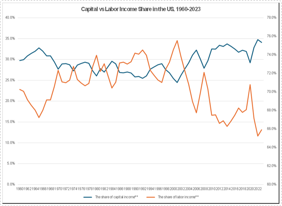
In the successive derivation above, we have assume that the profit share is fixed, resulting in the same constant labor income share in the national income. In the US economy, however, the estimated income share parameter has constantly shifted as the economy and various factors that affect the distribution of national income evolve over time. Inspired by Basu (2021)’s empirical study on this issue, the following chart (constructed from NIPA table 1.14) shows this historical evolution of the US economy expressed in terms of two income shares:
The same NIPA table also allows us to decompose the entire capital income into its detailed components such as retained earning, dividend payment, net interest payment, etc. For example, the following chart shows the types of capital income paid and distributed by the entire corporate business sector in the US.
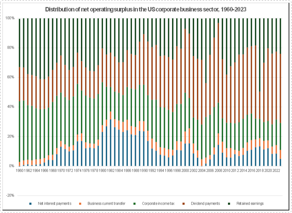
In the period from 1960 to the early 1980, retained earnings and taxes on corporate income make up the largest portion of capital income. Interest payments starts becoming quantitatively important since the early 1970s. From the early 1980s, the share of capital income taking the form of dividend payments has been on the rise, while corporate income tax has been falling. The share of capital income taking the form of retained earnings has been stable and significant. If we single out nonfinancial corporate business sector from the the entire corporate business sector, we can see that the interest income payment to the financial sector accounts for a much larger share of total capital income, which corresponds to the trend in the US economy that many non-financial corporate business firms have paid a greater share of their capital income to the financial sector since the early 1980s.
These two empirical compilations of macroeconomic data demonstrate that (1) the income distribution parameter in the US has changed over time and (2) even the internal distribution of capital income has been also shifted primarily because of the change in economic institutions and practice that affect the historical relationship between financial and non-financial corporate business sector.
If a growth model is designed to explain the long-run process of economic growth, any meaningful model designed to represent stylized facts of economic growth should be able to explain why this time-varying distributional outcomes come about in the first place. Unfortunately, the Solow growth models and later theoretical and empirical studies based upon his technology-augmented growth model have failed to account for this fundamental pattern.
An interactive visualization
An interactive visualization
Before closing this notebook, let us create an interactive chart that mimics the dynamic behavior of the solution curves in Solow’s technology-augmented growth model. This interactive chart is exactly the same as what we saw in the previous notebook, except this time that we also have introduced an option to plot a series of randomly generated data equivalent to output per effective worker alongside Solow’s prediction of output per effective worker. We can easily create this dataset by imposing the same mathematical operations to any variable.
For example, suppose we want to create a dataset whose x value goes from 1 to 10 while the corresponding y value is y(x) = gx^α where both g and α are constant. If g = 1 and α = 0.5, we get:
In[]:=
Clear[x,g,α];g=1;α=0.5;dataset=Table[{x,gx^α+RandomReal[{-1,1}]},{x,1,10}]
Out[]=
{{1,1.23044},{2,0.962766},{3,1.23035},{4,2.88497},{5,2.06464},{6,2.40097},{7,2.58094},{8,2.62501},{9,3.91902},{10,3.09159}}
In[]:=
ListPlot[dataset,PlotStyle->Red]
Notice that the function argument g x^α is the same as what the technology-augmented Solow growth model predicts. But the dataset just created is meaningless. It is just a result of a simple mathematical operation applied to the unknown variable x.
The following syntax allows us to show and control both Solow’s prediction about output per effective worker and this meaningless data point together:
Conclusion
Conclusion
The discussion in this notebook centers on one fundamental problem surrounding Solow’s technology-augmented production function. It is demonstrated that the Cobb-Douglas form of the aggregate production function is a mere result of successive algebraic derivations from the basic national income account identity, in which the A term is nothing more than the product of a weighted average of income distribution parameters and the constant of integration. In this algebraic formulation, the income distribution parameter is assumed to be constant throughout, which is not empirically supported by the real-world data. Interpreting this A term as if it is a proxy of the production technology is a gross intellectual mistake, while conducting cross-country regression studies using ‘growth accounting formula’ misled us, too. As an alternative, it is argued that any meaningful growth model must introduce a mechanism that explains the endogenous determination and distribution of national income.
Even in the face of this fundamental critique, many economists have continued to use Solow’s technology-augmented aggregate production in their modeling and econometric studies. The conventional practice for interpreting the A-term as a proxy of the evolution of the production technology is still prevailing in economics literature. The only possible innovation in this framework is to introduce some auxiliary variables that may explain the evolution of this A-term. We will see in the next session how Real Business Cycle (RBC) theorists introduce a stochastic disturbance term inside the A-term and present their simulation result as if it accounts for some stylized facts of economic growth patterns in the U.S.
Reference
Reference
◼
Anwar Shaikh, “Laws of Production and Laws of Algebra: The Humbug Production Function,” The Review of Economics and Statistics, Vol. 56, No. 1 (1974), pp.115-120.
◼
------------------, “Laws of Algebra and Laws of Production: Humbug II,” in Growth, Profits and Property: Essays in the Revival of Political Economy, edited by E. J. Nell, Cambridge, UK: Cambridge University Press, 1980, pp.80-95.
◼
------------------, “The Humbug Production Function,” in The New Palgrave: A Dictionary of Economic Theory and Doctrine, edited by J. Eatwell, M. Milgate, and P. Newman, London: Macmillan, 1987, pp.191-94.
◼
------------------, “Nonlinear Dynamics and Pseudo-Production Functions,” Eastern Economics Journal, Vol. 31, No. 3 (2005 ), pp.447-466.
◼
Deepankar Basu, The Logic of Capital - An Introduction to Marxist Economic Theory, Cambridge
and New York: Cambridge University Press, 2021.
and New York: Cambridge University Press, 2021.
◼
Jesus Felipe, and John McCombie, “The Tyranny of the Identity: Growth Accounting Revisited,” International Review of Applied Economics, Vol. 20, No. 3 (2006), pp.283-299.
◼
-----------------. “Aggregate Production Functions and the Accounting Identity Critiques: Further Reflections on Temple’s Criticisms and Misunderstandings,” Levy Economics Institute of Bard College Working Paper No. 718, Annandale-on-Hudson, New York: Levy Economics Institute, 2012.
◼
Robert Solow, “A Contribution to the Theory of Economic Growth,” The Quarterly Journal of Economics, Vol. 70, No. 1 (1956), pp.65-94.
◼
-----------------, “Technical Change and the Aggregate Production Function,” The Review of Economics and Statistics, Vol. 39, No. 3 (1957), pp.312-320.
CITE THIS NOTEBOOK
CITE THIS NOTEBOOK
Introduction to dynamic economic models: a classical Marxian critique of Solow's model
by Hee-Young Shin
Wolfram Community, STAFF PICKS, January 8, 2026
https://community.wolfram.com/groups/-/m/t/3602670
by Hee-Young Shin
Wolfram Community, STAFF PICKS, January 8, 2026
https://community.wolfram.com/groups/-/m/t/3602670