CITE THIS NOTEBOOK: Portfolio Optimization under Forecast-Informed Belief Revision by Danyang Chen. Wolfram Community JAN 13 2023.
Markowitz’s modern portfolio theory (MPT) is a widely used method for selecting the assets to maximize the return at a given level of risk. However, the MPT still produces relatively concentrated portfolios that emphasizing the assets performed well in the history. These assets will not necessarily perform well in the future and leads to potential losses and increased risk. We propose a new method by first using ARMA model to forecast the future daily returns, and then choose the averaged portfolio with highest Sharpe ratio predicted by MPT using the forecasted data. This method reduces the risk in the real market while keeping the return at the same level.
Introduction
Introduction
The Markowitz’s modern portfolio theory (MPT) [1] provides a way for risk-averse Investors to choose a portfolio by maximizing the return and/or minimizing the standard deviation (risk). As stated in Markowitz’s original paper, the MPT starts from the belief about the future risk and return but does not take the formation of the relevant beliefs into account. A simple way is to take the historical returns and standard deviations and use it as the belief for the future. Here we present a way of forming beliefs with ARMA forecasting and using them to produce more diversified portfolio that further reduce the risk.
Data Preparation
Data Preparation
Daily return of stocks from S&P500
Daily return of stocks from S&P500
We randomly draw 10 stocks from S&P500 index for portfolio construction. The date range is Jan. 1, 2013 to Jan. 1, 2021.
In[]:=
portfolio={"CSCO","PFE","DRI","CNC","GWW","FANG","EQR","STT","REG","TRV"};n=Length[portfolio];returns=TimeSeriesMap[Normal[#]&,#]&/@(FinancialData[#,"Return",{{2013,1,1},{2021,1,1}}]&/@portfolio);weights=Transpose[{Subscript[w,#]&/@portfolio}];
Mean return and risk
Mean return and risk
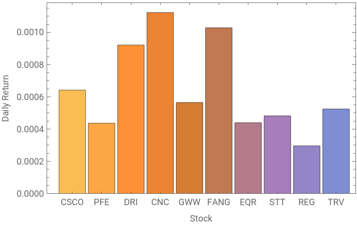
Return is computed from the daily change rate of the stock prices.
In[]:=
meanRet=Mean[#]&/@returns;BarChart[{meanRet},ChartLabelsportfolio,Frame->True,FrameLabel->{"Stock","Daily Return"}]
Out[]=
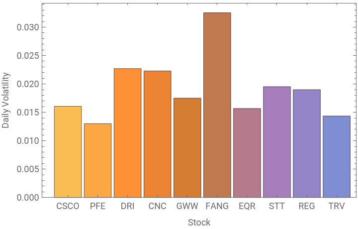
Risk is quantified using the standard deviation of the daily returns.
In[]:=
meanVol=StandardDeviation[#]&/@returns;BarChart[{meanVol},ChartLabelsportfolio,Frame->True,FrameLabel->{"Stock","Daily Volatility"}]
Out[]=
Correlation between stocks
Correlation between stocks
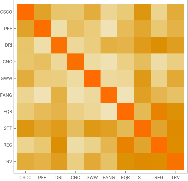
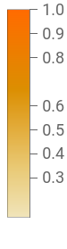
Correlation between stock prices are essential in MPT. If two stocks are highly correlated, combination of them does not significantly reduce the risk level. The benefits of MPT comes from choosing uncorrelated or even negatively correlated assets to reduce the overall risk level.
In[]:=
returnNormal=#["Values"]&/@returns;covMatrix=Covariance[Transpose[returnNormal]];correlation=Correlation[Transpose[returnNormal]];MatrixPlot[correlation,FrameTicks->{Thread[{Range[10],portfolio}]},PlotLegends->Automatic]
Out[]=
Portfolio Optimization
Portfolio Optimization
Portfolio return and risk
Portfolio return and risk
Based on the belief that the future performance of the asset is the same as history, we can calculate the portfolio return by
and the portfolio risk
Cw
μx
T
w
and the portfolio risk
2
σ
T
w
In[]:=
portfolioMean=Flatten[meanRet.weights][[1]];portfolioVar=Flatten[Transpose[weights].covMatrix.weights][[1]];
Efficient frontier
Efficient frontier
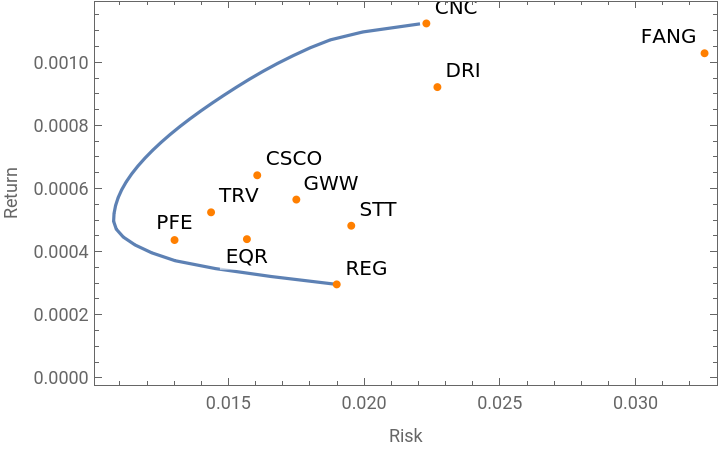
The efficient frontier, defined as the portfolio with the lowest risk for a given level of return. It could be obtained by minimizing the portfolio risk under the constraints for a given level of portfolio return
0≤≤1,i1,⋯,n
w
i
In[]:=
effFrontier=Table[{Sqrt[NMinimize[{portfolioVar,Union[GreaterEqualThan[0][#]&/@Flatten[Transpose[weights]],LessEqualThan[1][#]&/@Flatten[Transpose[weights]],List[Total[weights][[1]]1],List[Equal[portfolioMean,i]]]},Flatten[weights]][[1]]],i},{i,Min[meanRet],Max[meanRet],0.000025}];//Quiet
In[]:=
Show[ListLinePlot[effFrontier,PlotLegends->{"Efficient Frontier"}],ListPlot[MapThread[Labeled,{Thread[{meanVol,meanRet}],portfolio}],PlotStyle->Orange],FrameTrue,FrameLabel{"Risk","Return"},PlotRange->Automatic]
Out[]=

Portfolio optimization by maximizing the Sharpe ratio (tangent portfolio)
Portfolio optimization by maximizing the Sharpe ratio (tangent portfolio)
The tangent portfolio could be obtained by maximizing the Sharpe ratiowhere r is the risk free interest rate. The tangent portfolio has the highest ratio of return (deflated by ) to risk. The return and risk of the tangent portfolio is shown by the red point.
In[]:=
r=0.00004;(*Riskfreeratio*)psr=NMaximize[{(portfolioMean-r)/Sqrt[portfolioVar],Union[GreaterEqualThan[0][#]&/@Flatten[Transpose[weights]],LessEqualThan[1][#]&/@Flatten[Transpose[weights]],List[Total[weights][[1]]1]]},Flatten[weights]][[2]];
In[]:=
expRetRiskPsr={Sqrt[portfolioVar/.psr],portfolioMean/.psr};ListLinePlot[{effFrontier,{{0,r},expRetRiskPsr}},Epilog{Red,PointSizeLarge,Point[expRetRiskPsr]},FrameTrue,FrameLabel{"Risk","Return"}]
As shown in the following plot, the tangent portfolio is highly concentrated in three stocks, CNC, CSCO and DRI .
Alter future beliefs with ARMA forecasting
Alter future beliefs with ARMA forecasting
Change of optimal portfolio over time
Change of optimal portfolio over time
Future is not predictable. The risk and return are subject to changes due to market trends and company situations. If we look back in history and compute the tangent portfolio with data from the past year, it was significantly changing over time. The best portfolio in 2019 may perform terribly in 2020. Believing the assets to perform the same as in history is very risky.
Forecast-informed Portfolio using ARMA model
Forecast-informed Portfolio using ARMA model
We further reduce the risk by forming beliefs randomly with the ARMA model. These randomly generated beliefs could lead to many different tangent portfolios and we take the average of them as the forecast-informed portfolio.
The ARMA model (p=2 and q=2) is trained with mean return and covariance matrix from historical data.
The ARMA model (p=2 and q=2) is trained with mean return and covariance matrix from historical data.
Then we generate 50 simulations of future daily returns and obtains the tangent portfolio for each simulation.
The average of all tangent portfolio in simulations is taken as the forecast-informed portfolio. As shown below, this portfolio is much more diversified than the choice of MPT.
Backtest the forecast-informed portfolio
Backtest the forecast-informed portfolio
Now we test this portfolio for the real stock market from Jan. 1, 2021 to Jan. 1, 2023. The tangent portfolio and the forecast-informed portfolio are calculated at Jan. 1, 2021. We look at risk and return of these two portfolio in periods of 252 days between 2021 and 2023.
The following plot shows the risk and return of these two portfolios on the real data. We find that this forecast-informed portfolio has smaller risk comparing to the tangent portfolio while keeping the return at roughly the same level.
The Sharpe ratio is improved by
Concluding remarks
Concluding remarks
The belief that future return and risk are constant and equal to the historical values underestimates the overall risk and produces relatively concentrated portfolios. We improved the MPT by including such uncertainties in the market by simulating potential outcomes of the stock prices, and taking the averaged tangent portfolio evaluated from the simulated stock prices. This method produces much more diversified portfolio and has lower risk comparing to the tangent portfolios predicted by MPT. The use of the ARMA forecast model demonstrates the degree to which belief revision (in this case, as informed by an ARMA forecast), alters portfolio compositionally. And in this case, the forecast-informed portfolio appears to be better, with performance contingent upon the accuracy of the forecast.
Keywords
Keywords
◼
Modern portfolio theory
◼
ARMA model
◼
Risk management
Acknowledgment
Acknowledgment
I would like to thank James Boyd, Nik Murzin and Stephen Wolfram for valuable discussions and support for the winter school.
References
References
◼
Markowitz, H. (1952). Portfolio Selection. The Journal of Finance, 7(1), 77–91.