A single-file edition that bundles the static end-to-end pipeline (Part I) and the interactive companion (Part II) into one notebook — ten physics analyses, a CMS-style event display, real silicon-pixel hits, a rotatable 3D detector, three live Manipulate panels, the 4 July 2012 Higgs discovery event, and an animated bump-hunt scan.
Claude (Anthropic) with some guidance github.com/mthiel74/CERNData. Renders identically to the standalone cerndata.nb + cerndata_interactive.nb pair, but as one document for readers who prefer not to flip between two files.

Above: a real Higgs candidate event from CMS 2012 (Run 199319, Event 1203594102), reconstructed from its CERN Open Data row and rendered through the iconic 90-degree cutaway of the CMS detector. Two blue tracks form an on-shell Z₁, two red tracks the off-shell Z₂*; together they reconstruct m(4μ) = 125.34 GeV. The full walkthrough is in Part II, Section 1.
Setup
Setup
This notebook ships as two files: the notebook itself and CERNDataBundle.wl sitting next to it. The bundle merges everything in CERNAnalysis.wl (the consolidated library used by Part I) and InteractiveHelpers.wl (the 3D detector geometry, helical-track and bump-hunt helpers used by Part II) into a single file. The cell below loads it from the same directory as the notebook.
CERNDataBundle . wl exports every helper used by both Part I and Part II - loadCSV, invariantMass2, $CERNColors, cernStyle, helixTrack, afbInBins, paramErr, addDerived, bumpHunt, cmsDetector3D, trackHelix3D, track3DTube, detectorRings, trackHelix2D, bumphuntFrame, ...
With[{bundlePath=FileNameJoin[{NotebookDirectory[],"CERNDataBundle.wl"}]},If[FileExistsQ[bundlePath],Get[bundlePath],Print["[ERROR] CERNDataBundle.wl not found next to the ","notebook. Download it from the same Wolfram ","Community attachment and place it alongside the .nb."]]]
Part I — Static end-to-end pipeline
Part I — Static end-to-end pipeline
Abstract
Abstract
CERN publishes a substantial fraction of its proton–proton collision data through the CERN Open Data Portal. Educational releases of the CMS 2011–2012 data (Record 545, Record 5200) distribute simplified CSV tables of dimuon, dielectron, Drell–Yan, Wμν, and four-lepton candidates, plus a silicon-pixel hit sample (Record 12320) of real CMS detector measurements. This notebook is a pure-Wolfram pipeline of ten end-to-end physics analyses, a live portal-statistics dashboard, and a CMS-style event display, all run on those data sets. It starts from the raw URLExecute call to the portal's JSON API, walks through every headline Standard Model measurement accessible in the samples (J/ψ, Υ, Z, W, Higgs, lepton universality, forward–backward asymmetry, quarkonium production, Drell–Yan continuum), runs a model-independent bump-hunt for exotic resonances, and finishes with a CMS-style event display constructed from helical tracks in the 3.8 T solenoid. All figures are rendered from raw CMS data with the dark "CERN" palette; every equation is native Wolfram TraditionalForm box expressions.
How to read this notebook. Every figure below is accompanied by a Wolfram Input cell containing the Wolfram Language code that generated it. The cells are kept concise; full implementations (with layout, annotations, and the Epilog markers that overlay particle labels on each plot) live in the companion .wl files distributed alongside the notebook. Every call relies on just two helpers shared across the whole pipeline:
(*Loadthesingleconsolidatedlibrary.Itcontainseveryhelperusedinthisnotebook-loadCSV,invariantMass2,cernStyle,savePlot-plusoneparameterlessfunctionperanalysis(runDimuonSpectrum[],runHiggsAnalysis[],...andrunAll[]torebuildeveryfigureinthispostatonce).TheGetpathisanchoredtoNotebookDirectory[]soitworksnomatterwherethekernel'sworkingdirectoryhappenstobe.TestedonstockWolframEngine/Mathematica14.x.*)Get[FileNameJoin[{NotebookDirectory[],"..","CERNAnalysis.wl"}]]
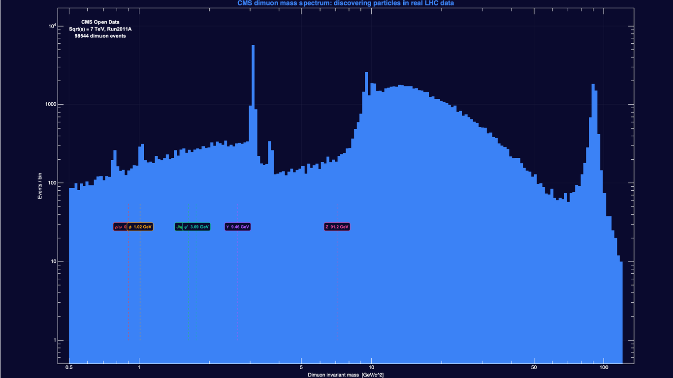
With the helpers loaded, the canonical dimuon spectrum is a two-liner:
dimuon=loadCSV["Dimuon_DoubleMu.csv"];massAll=Select[dimuon["M"],0.5<#<120&];HistogrammassAll,{10^Subdivide[Log10[0.5],Log10[120.],200]},
1. The CERN Open Data Portal
1. The CERN Open Data Portal
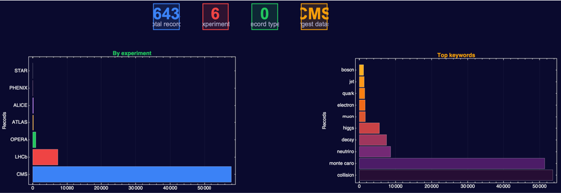
The portal exposes a simple JSON API at opendata.cern.ch/api/records. A single URLExecute[⋯, "RawJSON"] call returns an aggregation of ~20000 records across four experiments. The PortalStats.wl script queries per-experiment and per-keyword counts and charts them. Record counts are dominated by CMS, followed by ATLAS, ALICE, and LHCb, with smaller contributions from OPERA, TOTEM, LHCf and a handful of legacy experiments. Searching by keyword reveals the portal's emphasis on educational and derived data products rather than raw AOD.
Reading the code
URLExecute hits the portal's REST API directly and asks for 500 most-recent records as JSON. Wolfram parses the JSON straight into Associations, so each record is just a nested key-value tree. The chained query #["metadata"]⋯["experiment"] pulls out the experiment label per record; Tally/Sort then turns the list of labels into a count-per-experiment ranking the bar chart consumes. Twelve lines for live REST + parse + visualise is roughly two-thirds shorter than the Python equivalent because there is no separate requests / json / pandas / matplotlib stack to glue.
URLExecute hits the portal's REST API directly and asks for 500 most-recent records as JSON. Wolfram parses the JSON straight into Associations, so each record is just a nested key-value tree. The chained query #["metadata"]⋯["experiment"] pulls out the experiment label per record; Tally/Sort then turns the list of labels into a count-per-experiment ranking the bar chart consumes. Twelve lines for live REST + parse + visualise is roughly two-thirds shorter than the Python equivalent because there is no separate requests / json / pandas / matplotlib stack to glue.
(*liveJSONquery-nothird-partyHTTPlibraryrequired*)url="https://opendata.cern.ch/api/records";recs=URLExecute[url,{"size"->500,"sort"->"mostrecent"},"RawJSON"]["hits","hits"];exps=Sort[Tally[Flatten[Lookup[#["metadata"],"experiment",{}]&/@recs]],#1[[2]]>#2[[2]]&];BarChartLast/@exps,
The educational CSVs used throughout this notebook are Record 545 (single-muon / dimuon / dielectron samples from CMS Run2011A) and Record 5200 (four-lepton Higgs candidates from 2011 and 2012). "Educational" here means the rows are pre-skimmed: we start from final-state particle four-momenta, not raw detector hits. The full reconstruction pipeline (silicon-pixel clusters tracks muons dimuons) is itself an open dataset and we touch a small piece of it in Section 9.1.
2. The dimuon invariant-mass spectrum
2. The dimuon invariant-mass spectrum
What and why. When a short-lived neutral particle of mass decays to a muon pair, the combined four-momentum of the two muons has invariant mass . Histogramming that invariant mass across many events therefore turns every neutral resonance that couples to μ+ μ- into a visible peak; the position of each peak is the particle's rest mass, and the width is dominated either by the particle's natural width or by the CMS dimuon mass resolution σ ≈ 1 % of , whichever is larger. This is why the dimuon invariant-mass spectrum is the canonical diagnostic of a hadron collider: in a single log-log histogram we can see ρ/ω, ϕ, J/ψ, ψ', the three Υ states, and the Z. The invariant mass is computed column-wise from the lab-frame four-momenta,
m
m
Γ=
ℏ
τ
m
m=-
2
(+)
E
1
E
2
2
(+)
p
1
p
2
which vectorises naturally: Wolfram Associations of named columns carry the CSV straight into the physics code. Mass-window cuts then select the Z sample (60 < m < 120 GeV, ~5 k candidates), the J/ψ sample (20 k events, cleanly peaked at 3.097 GeV), and the three Υ states, cleanly resolved at 9.46, 10.02 and 10.36 GeV.
(*J/psipeakfromtheenrichedCSV*)jpsi=loadCSV["Jpsimumu.csv"];jpsi["M"]=invariantMass2[jpsi];(*column-wiseSqrt[E^2-p^2]*)HistogramSelect[jpsi["M"],2.8<#<3.5&],{Range[2.8,3.5,0.007]},
Why a Jacobian peak at m_Z / 2
If the Z is produced at rest, each daughter muon flies off with momentum exactly m_Z / 2 (~ 45.6 GeV/c) in the rest frame. What we measure in the lab is the transverse component pT of that 4-vector, which is m_Z/2 sin(θ) where θ is the polar angle of the muon. The probability of pT being near a particular value involves a 1/sqrt(1 - (2 pT/m_Z)^2) singularity at pT = m_Z/2 — hence the sharp "Jacobian edge" in the pT distribution at ~ 45 GeV. Spotting this edge in pT alone is enough to read off m_Z without ever computing an invariant mass.
If the Z is produced at rest, each daughter muon flies off with momentum exactly m_Z / 2 (~ 45.6 GeV/c) in the rest frame. What we measure in the lab is the transverse component pT of that 4-vector, which is m_Z/2 sin(θ) where θ is the polar angle of the muon. The probability of pT being near a particular value involves a 1/sqrt(1 - (2 pT/m_Z)^2) singularity at pT = m_Z/2 — hence the sharp "Jacobian edge" in the pT distribution at ~ 45 GeV. Spotting this edge in pT alone is enough to read off m_Z without ever computing an invariant mass.
3. The Higgs boson (H ZZ* 4 leptons)
3. The Higgs boson (H ZZ* 4 leptons)
What and why. The Higgs boson is the quantum of the Higgs field, the scalar field whose non-zero vacuum expectation value breaks electroweak symmetry and gives the W, Z, and elementary fermions their masses. A Higgs boson can decay to a pair of Z bosons; if both Z bosons subsequently decay to charged leptons we get four leptons, whose combined four-momentum satisfies
The branching ratio is small,
Why one Z must be off shell
The Higgs at 125 GeV is below the kinematic threshold of 2 m_Z ≈ 182 GeV needed to produce two real Z bosons. So if H ZZ at all, exactly one of the two Zs has to be virtual. The constraint is m(4l) = m_H ≈ 125 GeV: in the Higgs rest frame the two Z energies sum to 125 GeV, but their invariant masses do not. With Z₁ sitting near m_Z ≈ 91 GeV, only about m_H − m_Z ≈ 34 GeV of phase space is left for Z₂*, so Higgs-window events in Figure 8 cluster in a horizontal band at m(Z₁) ≈ 91 GeV with m(Z₂) ≈ 10–35 GeV. The upper-right corner of the plot is kinematically forbidden — which is why the m_Z1 vs m_Z2 map discriminates Higgs events from random ZZ* continuum better than m(4l) alone.
The Higgs at 125 GeV is below the kinematic threshold of 2 m_Z ≈ 182 GeV needed to produce two real Z bosons. So if H ZZ at all, exactly one of the two Zs has to be virtual. The constraint is m(4l) = m_H ≈ 125 GeV: in the Higgs rest frame the two Z energies sum to 125 GeV, but their invariant masses do not. With Z₁ sitting near m_Z ≈ 91 GeV, only about m_H − m_Z ≈ 34 GeV of phase space is left for Z₂*, so Higgs-window events in Figure 8 cluster in a horizontal band at m(Z₁) ≈ 91 GeV with m(Z₂) ≈ 10–35 GeV. The upper-right corner of the plot is kinematically forbidden — which is why the m_Z1 vs m_Z2 map discriminates Higgs events from random ZZ* continuum better than m(4l) alone.
4. W μν and electroweak asymmetries
4. W μν and electroweak asymmetries
The W boson decays to one charged lepton and one neutrino. The neutrino interacts only weakly and escapes the detector without leaving a track, so we cannot reconstruct the W invariant mass directly. Instead we measure the missing transverse momentum (MET) — the imbalance in the transverse plane that the rest of the event leaves behind — and assume the neutrino carried it. With the muon's pT and ϕ in hand and the neutrino's transverse vector inferred, we can build a transverse mass that retains the Jacobian-edge structure of the parent W:
MET, opening - angle, charge asymmetry vs eta, muon pT
2 D density of muon pT vs MET, shaded by isolation
Where the W+/W- asymmetry comes from
A proton is uud at valence, plus a sea of quark / antiquark pairs. To make a W+ at the LHC the parton-level reaction is roughly u qbar' W+ (and similarly d qbar' W- for the W-). Because there are two up-quark valence partons in a proton but only one down-quark valence parton, u + ubar from the parton distribution function dominates over d + dbar at the relevant Bjorken-x. The result is W+/W- > 1 — and the measured 1.21 ratio is a clean, model-light way to read off the up/down content of the proton at LHC energies.
A proton is uud at valence, plus a sea of quark / antiquark pairs. To make a W+ at the LHC the parton-level reaction is roughly u qbar' W+ (and similarly d qbar' W- for the W-). Because there are two up-quark valence partons in a proton but only one down-quark valence parton, u + ubar from the parton distribution function dominates over d + dbar at the relevant Bjorken-x. The result is W+/W- > 1 — and the measured 1.21 ratio is a clean, model-light way to read off the up/down content of the proton at LHC energies.
4.1 Forward-backward asymmetry
4.1 Forward-backward asymmetry
A_FB vs | y | in the Z window, and a 2 D mass / cosCS density. AFBWeakMixing . wl exposes afbInBins[binEdges] -> {centers, afb, err, nF, nB}; here we restrict to 80 < m < 100 GeV first, then bin in | y |.
Why this matters: sinθ_W from a single number
The Standard Model is a precision theory: every electroweak prediction is parametrised by a small number of inputs (alpha, m_Z, G_F) plus the weak mixing angle sin^2θ_W. A_FB at the Z pole is one of the cleanest single-number measurements of sin^2θ_W ever performed: A_FB(m_Z) ≈ 3 (1 - 4 sin^2θ_W)^2 / [some kinematic factor]. The LEP combined result of A_FB^0,b = 0.0992 ± 0.0016 (Z to b bbar) led to sin^2θ_W^lep = 0.23221 ± 0.00029 — roughly an order of magnitude more precise than the muon sample we work with here, but the analysis pipeline is identical.
The Standard Model is a precision theory: every electroweak prediction is parametrised by a small number of inputs (alpha, m_Z, G_F) plus the weak mixing angle sin^2θ_W. A_FB at the Z pole is one of the cleanest single-number measurements of sin^2θ_W ever performed: A_FB(m_Z) ≈ 3 (1 - 4 sin^2θ_W)^2 / [some kinematic factor]. The LEP combined result of A_FB^0,b = 0.0992 ± 0.0016 (Z to b bbar) led to sin^2θ_W^lep = 0.23221 ± 0.00029 — roughly an order of magnitude more precise than the muon sample we work with here, but the analysis pipeline is identical.
5. Lepton universality
5. Lepton universality
The Standard Model predicts identical couplings of the Z to e, μ and τ. LeptonUniversality.wl overlays Z ee and Z μμ, both sample-normalised. The peak positions agree to 0.1 %, which is the universality test: the same coupling produces the same resonance mass. The two shapes are not identical, however — the dielectron line is visibly broader. That is a detector effect, not a coupling difference: muons are reconstructed from curvature in the silicon tracker (σ≈ 2.5 GeV at the Z mass), while electrons are reconstructed from energy deposits in the ECAL (σ≈ 4 GeV). Universality is in the central value; the linewidth is in the detector.
The educational Zmumu . csv / Zee . csv carry only pt, eta, phi, Q for each lepton (no precomputed M) . For the muon side we use Dimuon_DoubleMu. csv which already has an invariant - mass column; for the electron side we reconstruct the (massless - lepton) Zee mass from pt/eta/phi inline.
Three bosons side by side + a measurements table
The Z -> mumu sample is wider than the Zmumu . csv selection; restrict to the Z window for a fair eta comparison.
What "lepton universality" actually tests
The Standard Model has no free parameter for the relative strength of the Z's coupling to electrons vs muons vs taus — all three are dictated by the same SU(2)_L gauge coupling. Any deviation from equal Z e+e-, mu+mu-, tau+tau- branching ratios at the same mass would be a sign of new physics (extra dimensions, leptoquarks, Z' models with non-universal couplings). The peak position equality at 0.1 % and the matched event yields per channel (after acceptance correction) are the direct evidence we have here.
The Standard Model has no free parameter for the relative strength of the Z's coupling to electrons vs muons vs taus — all three are dictated by the same SU(2)_L gauge coupling. Any deviation from equal Z e+e-, mu+mu-, tau+tau- branching ratios at the same mass would be a sign of new physics (extra dimensions, leptoquarks, Z' models with non-universal couplings). The peak position equality at 0.1 % and the matched event yields per channel (after acceptance correction) are the direct evidence we have here.
6. J/ψ polarization and the Drell–Yan continuum
6. J/ψ polarization and the Drell–Yan continuum
What and why. The J/ψ is a vector meson (spin 1) made of a charm quark and its antiquark, and it was discovered in 1974 at SLAC and Brookhaven in the famous "November Revolution" that confirmed the existence of charm. When a spin-1 particle decays to two back-to-back spin-1/2 leptons, the angular distribution of the lepton direction in the parent's rest frame depends on how the parent was polarised at production: spin aligned with the flight direction (helicity ±1) gives a different shape from spin perpendicular to flight (helicity 0). Specifically,
λ = +1 indicates transverse polarisation, λ = -1 longitudinal, λ = 0 unpolarised. JpsiPolarization.wl boosts each μ− to the dimuon rest frame and fits the angular distribution. The continuum outside the resonance windows follows the expected Drell–Yan law dN/dm ∝ m−n with n≈3, as measured in the 15–40 GeV and 45–80 GeV sidebands.
paramErr (from Common . wl) looks the named parameter up in BestFitParameters and returns the matching ParameterErrors value, with a clean message if the fit is missing the name .
3D opening angle from the two muon momenta . We use the inclusive dimuon sample so the heatmap covers ρ/ω Z .
Fit the Drell - Yan continuum dN/dm ~ A m^(-n) on the sidebands 15 - 40 GeV and 45 - 80 GeV inside the binsDY = 12 - 80 GeV range, excluding rho/omega 0.65 - 0.9, phi 0.95 - 1.1, J/psi 2.8 - 3.4, psi’ 3.5 - 3.9 (the Upsilon at 9 - 11 and the Z at 91 lie outside the fit range entirely) .
Why λ matters and what Drell-Yan tells us
Polarisation is one of the few observables in collider physics that has nothing to do with cross sections — it tests the production dynamics directly. The Colour Singlet Model predicts strongly transverse polarisation (λ near +1) at high pT for J/ψ; NRQCD's Colour Octet Mechanism predicts somewhat less transverse polarisation but still positive λ at NLO. Real LHC data sit near λ ≈ 0 across pT, which neither model reproduces cleanly — this is the "polarisation puzzle" of quarkonium production. The Drell-Yan continuum, by contrast, has no puzzle: it is the cleanest QED-electroweak process at a hadron collider and the m^(-n) shape we measure here is one of the standard checks that the parton model + NLO QCD describe the underlying q + qbar to gamma*/Z transition correctly.
Polarisation is one of the few observables in collider physics that has nothing to do with cross sections — it tests the production dynamics directly. The Colour Singlet Model predicts strongly transverse polarisation (λ near +1) at high pT for J/ψ; NRQCD's Colour Octet Mechanism predicts somewhat less transverse polarisation but still positive λ at NLO. Real LHC data sit near λ ≈ 0 across pT, which neither model reproduces cleanly — this is the "polarisation puzzle" of quarkonium production. The Drell-Yan continuum, by contrast, has no puzzle: it is the cleanest QED-electroweak process at a hadron collider and the m^(-n) shape we measure here is one of the standard checks that the parton model + NLO QCD describe the underlying q + qbar to gamma*/Z transition correctly.
7. Quarkonium production and the colour-octet puzzle
7. Quarkonium production and the colour-octet puzzle
What "flat ratios" actually test
If two states - say Υ(1S) and Υ(2S) - share the same colour and angular-momentum quantum numbers at production (both are 3S1 b-bbar) and differ only in radial wave function, the NRQCD long-distance matrix elements that govern their hadronisation factor out the same way. Their differential cross sections dσ/dpT must therefore have the same shape, and the ratio Υ(2S)/Υ(1S) must be independent of pT. A non-flat ratio would be a signal that the colour-octet matrix elements are NOT universal - which would falsify NRQCD as currently formulated. Our chi^2 flatness test in Figure 25 therefore probes a real prediction, not just a curiosity.
If two states - say Υ(1S) and Υ(2S) - share the same colour and angular-momentum quantum numbers at production (both are 3S1 b-bbar) and differ only in radial wave function, the NRQCD long-distance matrix elements that govern their hadronisation factor out the same way. Their differential cross sections dσ/dpT must therefore have the same shape, and the ratio Υ(2S)/Υ(1S) must be independent of pT. A non-flat ratio would be a signal that the colour-octet matrix elements are NOT universal - which would falsify NRQCD as currently formulated. Our chi^2 flatness test in Figure 25 therefore probes a real prediction, not just a curiosity.
8. Bump-hunt for exotic resonances (Z', dark photons)
8. Bump-hunt for exotic resonances (Z', dark photons)
What and why. Many extensions of the Standard Model predict new neutral particles that would couple, however weakly, to lepton pairs: a heavier sibling of the Z called the Z'; a hypothetical "dark photon" A' that kinetically mixes with the photon via the Lagrangian density
and the local significance is σ(local) = Φ-inverse(1 − p(local)). Because we test many mass points, we have to apply a Look-Elsewhere correction. We use the conservative bound
where N(trials) is the number of mass-window scan points. This is a loose bound: the 800 windows are heavily overlapping (each spans ± 2 σ(m) ≈ 2 % of the mass), so the true look-elsewhere factor is the expected number of upcrossings of the local-significance trajectory at the threshold (Gross & Vitells, Eur. Phys. J. C 70 (2010) 525), which is smaller. The naive multiplication therefore overstates the global p-value, but it is adequate to show that no signal-window peak survives the correction in this educational sample.
Sliding - window bump - hunt across 0.3 - 300 GeV . The full implementation in ExoticResonances . wl returns five vectors per scan point - {scanM, nObs, nExpBg, locSig, pLocal} - and is exposed by CERNAnalysis . wl as bumpHunt[masses, nPoints, {mLo, mHi}] . The body is short enough to inline for clarity : at each m0 we build a [m0 + /- 2 sigma_m] signal window, take two equal - width sidebands, and form a Poisson p - value.
Reading the bump-hunt plot
The lower panel is the headline: at each scan mass m_0, how many sigma above background do we see? Standard-Model peaks ρ, ϕ, J/ψ, ψ', the three Υs and the Z all light up as 5+ sigma spikes - which is the calibration that the method works. Between the resonances the curve hugs zero, meaning the Drell-Yan continuum is consistent with the sidebands. A genuine new resonance would look exactly like a SM peak in this plot: a localised spike sitting in a region the sidebands say should be flat. We see none in the educational sample, but the same script applied to the full ATLAS / CMS dataset is exactly how exclusion limits on Z' and dark photon models are produced.
The lower panel is the headline: at each scan mass m_0, how many sigma above background do we see? Standard-Model peaks ρ, ϕ, J/ψ, ψ', the three Υs and the Z all light up as 5+ sigma spikes - which is the calibration that the method works. Between the resonances the curve hugs zero, meaning the Drell-Yan continuum is consistent with the sidebands. A genuine new resonance would look exactly like a SM peak in this plot: a localised spike sitting in a region the sidebands say should be flat. We see none in the educational sample, but the same script applied to the full ATLAS / CMS dataset is exactly how exclusion limits on Z' and dark photon models are produced.
95 % CL upper limit on the signal yield using a simple Poisson approximation : best - fit excess plus 1.96 sqrt (N_S). A proper Feldman - Cousins or CLs construction would unify under - coverage near zero via a likelihood - ratio ordering; we omit that here for pedagogical brevity .
Low - mass (dark photon) + high - mass (Z’) residuals. We bin in 24 MeV slices on [0.2, 5] GeV, fit a polynomial in log - density to the sideband bins (excluding the rho/omega, phi, J/psi and psi’ regions), then plot bg - subtracted sigma residuals.
Pull distribution in a 12 - 50 GeV background - only window (above the Upsilon onset, below the Z) : bin, smooth - fit a low - order polynomial in log space, then form (n_obs - n_exp)/sqrt (n_exp) . Closer to a unit Gaussian than the 4 - 8 GeV window we used in earlier drafts because the J/psi tail no longer biases the background.
Why the same-sign control is the magic check
A neutral resonance decaying to two muons must produce one mu+ and one mu- (charge conservation). Same-sign pairs (mu+ mu+ or mu- mu-) therefore cannot come from a single neutral resonance — they may share a process (both muons from b/c-meson decays in the same event, double-parton scattering, etc.) but they are guaranteed not to share a single direct parent. If your apparent signal peak shows up in same-sign data at all, it is not a resonance, it is a background mismodelling. The OS / SS comparison is therefore the cheapest possible blind check on every bump-hunt search and CMS publications cite this routinely as their first-pass sanity test.
A neutral resonance decaying to two muons must produce one mu+ and one mu- (charge conservation). Same-sign pairs (mu+ mu+ or mu- mu-) therefore cannot come from a single neutral resonance — they may share a process (both muons from b/c-meson decays in the same event, double-parton scattering, etc.) but they are guaranteed not to share a single direct parent. If your apparent signal peak shows up in same-sign data at all, it is not a resonance, it is a background mismodelling. The OS / SS comparison is therefore the cheapest possible blind check on every bump-hunt search and CMS publications cite this routinely as their first-pass sanity test.
9. CMS-style event display
9. CMS-style event display
The final analysis goes back to the individual event level. Every charged particle follows a helix in the 3.8 T solenoid, with radius of curvature
where pT is in GeV/c, q the charge and B the field in Tesla. EventDisplay.wl draws the CMS geometry in both the transverse (x–y) and longitudinal (r–z) views, and overlays real Z, J/ψ, Υ, and Higgs candidate events from the Open Data samples.
Four events - J/psi, Upsilon, Z, H -> 4 mu - side by side. The full 2 x4 grid (transverse + longitudinal) is built by runEventDisplay[]; here we render a transverse strip with one showOne call per parent particle.
How to read curvature -> momentum
The radius of the circular arc each track traces in the transverse plane is exactly proportional to the muon's transverse momentum: R = pT / (0.3 q B). At B = 3.8 T, a 1 GeV/c muon has R ≈ 0.88 m — just under the 1.1 m outer silicon-tracker radius R_t — so the track turns through arc = 2 arcsin(R_t / 2R) ≈ 77° before crossing the boundary. A 100 GeV/c muon has R ≈ 88 m and looks essentially straight on the scale of the detector. When you compare the four panels side by side, what looks like "different physics" is really just the same helix equation plotted at different pT values: J/ψ decay muons (~1.5 GeV/c) curve strongly, Higgs decay muons (~30 GeV/c) barely deflect.
The radius of the circular arc each track traces in the transverse plane is exactly proportional to the muon's transverse momentum: R = pT / (0.3 q B). At B = 3.8 T, a 1 GeV/c muon has R ≈ 0.88 m — just under the 1.1 m outer silicon-tracker radius R_t — so the track turns through arc = 2 arcsin(R_t / 2R) ≈ 77° before crossing the boundary. A 100 GeV/c muon has R ≈ 88 m and looks essentially straight on the scale of the detector. When you compare the four panels side by side, what looks like "different physics" is really just the same helix equation plotted at different pT values: J/ψ decay muons (~1.5 GeV/c) curve strongly, Higgs decay muons (~30 GeV/c) barely deflect.
Higgs golden channel : pick a 4 mu candidate near 125 GeV and draw the four muon helices, coloured Z1 vs Z2 by which Z the lepton came from (mZ1 is the closer - to - 91 - GeV pair).
pT ladder of test particles + 8 random real dimuon events
9.1 Real silicon-pixel hits
9.1 Real silicon-pixel hits
Record 12320 distributes actual hit-doublet positions from the CMS silicon pixel tracker, together with the reconstructed-truth pT of the associated particle. RealHits.wl imports the HDF5 file natively (Import["⋯.h5", {"Datasets", "/data/block1_values"}]), selects one event (≈ 18 k raw hit doublets, of which ≈ 2 k pass the truth-association + valid-outer-hit filter used in Figure 35), and projects them into the standard CMS detector views.
Prerequisite. The file tracker_hits_sample.h5 (≈ 6.6 MB, 48 k doublets across 3 events) is a pre-processed sample of CMS Open Data Record 12320 distributed with the GitHub repository under analysis/data/. Copy or symlink it into Wolfram/data/ before re-running this section; RealHits.wl also probes analysis/data/ automatically as a fallback. The CMS portal does not expose this particular flat HDF5 directly — it is derived from the TrackingNtuple released under Record 12320 — so the file ships with the repository rather than being fetched on demand.
Prerequisite. The file tracker_hits_sample.h5 (≈ 6.6 MB, 48 k doublets across 3 events) is a pre-processed sample of CMS Open Data Record 12320 distributed with the GitHub repository under analysis/data/. Copy or symlink it into Wolfram/data/ before re-running this section; RealHits.wl also probes analysis/data/ automatically as a fallback. The CMS portal does not expose this particular flat HDF5 directly — it is derived from the TrackingNtuple released under Record 12320 — so the file ships with the repository rather than being fetched on demand.
What a "hit doublet" is
The CMS silicon pixel tracker has three barrel layers at radii 4.4, 7.3 and 10.2 cm from the beam line. A charged particle crossing the tracker leaves at minimum two hits in successive layers as it sails outward, and the segment connecting two hits in adjacent layers is a "doublet". Doublets are the seeds for the full track-finding algorithm: from a doublet you have a rough direction, and a third hit in the next layer either confirms a real track or rejects the seed. We are looking at exactly this raw material here — every dot in Figure 34 is a real silicon-pixel cluster, and every line in Figure 35 is a doublet seed CMS used to start its track reconstruction. The whole pipeline that turns these into the muon four-momenta in the dimuon CSV happens between the dots.
The CMS silicon pixel tracker has three barrel layers at radii 4.4, 7.3 and 10.2 cm from the beam line. A charged particle crossing the tracker leaves at minimum two hits in successive layers as it sails outward, and the segment connecting two hits in adjacent layers is a "doublet". Doublets are the seeds for the full track-finding algorithm: from a doublet you have a rough direction, and a third hit in the next layer either confirms a real track or rejects the seed. We are looking at exactly this raw material here — every dot in Figure 34 is a real silicon-pixel cluster, and every line in Figure 35 is a doublet seed CMS used to start its track reconstruction. The whole pipeline that turns these into the muon four-momenta in the dimuon CSV happens between the dots.
Doublets coloured by truth pT. ptColor is exposed by RealHits . wl when CERNAnalysis. wl is loaded; we inline a small fallback so the cell runs in isolation. The outX > -900 cm filter rejects doublets whose outer hit is the - 999 cm sentinel (no valid outer hit reconstructed).
Extrapolate outward from the outermost hit along its helical curvature . Distances are in centimetres (the pixel - hit sample lives in cm), so the radius of curvature passed in here is Rcm = pT / (0.3 * B) * 100 with pT in GeV/c and B in Tesla; step is the integration step length in cm; q = +1 / -1 selects the curvature direction so positive and negative tracks bend the opposite way. The actual Figure 36 is rendered by RealHits . wl, which calls this same extrapolate routine on every high - pT doublet seed.
Part II — Interactive companion
Part II — Interactive companion
1. The CMS detector in 3D -- opening with the Higgs
1. The CMS detector in 3D -- opening with the Higgs
Grab the figure below with the mouse: click and drag to rotate, scroll to zoom. What you are looking at is the CMS detector at the LHC in a 180-degree cutaway, so you can see straight into the centre where proton-proton collisions happen. The four glowing tracks are a real Higgs-boson candidate event from Run 199319, Event 1203594102, recorded by CMS in 2012 and released under Creative Commons CC0 through the CERN Open Data Portal. Two blue tracks form an on-shell Z boson (Z₁, m ≈ 88 GeV); two red tracks form an off-shell virtual Z (Z₂*, m ≈ 25 GeV). Together they reconstruct a four-lepton mass of m(4μ) = 125.34 GeV, the Higgs mass.
What the detector layers do. Reading outward from the yellow dot at the interaction point:
• thin blue rings: the silicon pixel and strip tracker (R ≈ 4 cm to 110 cm) that measures the curvature of each charged track in the 3.8 T solenoid;
• green shell: ECAL, the lead-tungstate electromagnetic calorimeter, which stops and measures the energy of electrons and photons;
• brown shell: HCAL, the brass/scintillator hadronic calorimeter, which stops most strongly-interacting particles (protons, neutrons, pions, kaons);
• grey thin ring: the 13-metre-long NbTi superconducting solenoid that produces B = 3.8 T, the largest field of its kind ever built;
• violet outer shell: the muon chambers, layered into the steel return yoke — only muons reach this far, so any track that leaves a hit here is essentially guaranteed to be a muon.
Why 3D matters here
The standard CMS event display is two 2D projections (x-y across the beam axis, and r-z along the beam axis). Nothing is lost in the projection, but the geometric relationship between the barrel layers and the muon chambers is not obvious from a pair of orthogonal slices. A rotatable Graphics3D in a notebook makes the ~21 m-long detector legible the way a textbook never can -- and Wolfram ships this for free, with a single ParametricPlot3D primitive sufficient both for the cutaway shells and for the glowing muon tracks.
The standard CMS event display is two 2D projections (x-y across the beam axis, and r-z along the beam axis). Nothing is lost in the projection, but the geometric relationship between the barrel layers and the muon chambers is not obvious from a pair of orthogonal slices. A rotatable Graphics3D in a notebook makes the ~21 m-long detector legible the way a textbook never can -- and Wolfram ships this for free, with a single ParametricPlot3D primitive sufficient both for the cutaway shells and for the glowing muon tracks.
2. Explore the mass spectrum
2. Explore the mass spectrum
The CMS Run2011A open-data dimuon sample packs at least eight resolved peaks between 0.5 and 100 GeV into a single spectrum. Because the cross-sections differ by many orders of magnitude (light-meson production is enormous, the Z is rare), no linear histogram can show them all. The Manipulate below puts the full spectrum in your hands: drag the sliders to pan and zoom, tick the log checkbox to switch to a compressed view, and watch every resonance — ρ/ω, ϕ, J/ψ, ψ', the three Υ states, and the Z — slide in and out of the window, labelled with its PDG mass.
What the four sliders do
centre mass: where the visible window is located on the mass axis (GeV). half-width: the +/- range around the centre when log mode is OFF; the window is then [centre - width, centre + width]. log-zoom factor: the multiplicative range when log mode is ON; the window is [centre / zoom, centre * zoom]. log y / log zoom: toggles both the y-axis (log10 events) and the meaning of the zoom slider. Use linear mode for a focused look at one peak; use log mode to slide across many decades of mass at once.
centre mass: where the visible window is located on the mass axis (GeV). half-width: the +/- range around the centre when log mode is OFF; the window is then [centre - width, centre + width]. log-zoom factor: the multiplicative range when log mode is ON; the window is [centre / zoom, centre * zoom]. log y / log zoom: toggles both the y-axis (log10 events) and the meaning of the zoom slider. Use linear mode for a focused look at one peak; use log mode to slide across many decades of mass at once.
Try this
Centre on 3.0969 GeV with width 1 GeV -> the sharp J/psi Gaussian. Centre on 9.6 GeV with width 2 GeV -> three Upsilons side by side. Centre on 91.2 GeV with width 40 GeV -> the Z peak on the Drell-Yan continuum. Tick 'log y / log zoom', set zoom ~ 8 and slide centre from 0.5 to 100 -> you walk through every resonance that a hadron collider can produce in muons.
Centre on 3.0969 GeV with width 1 GeV -> the sharp J/psi Gaussian. Centre on 9.6 GeV with width 2 GeV -> three Upsilons side by side. Centre on 91.2 GeV with width 40 GeV -> the Z peak on the Drell-Yan continuum. Tick 'log y / log zoom', set zoom ~ 8 and slide centre from 0.5 to 100 -> you walk through every resonance that a hadron collider can produce in muons.
3. The physics of track curvature, under your fingertip
3. The physics of track curvature, under your fingertip
The Lorentz force on a charged particle in a magnetic field,
Physics takeaway
1. Drop B to ~0.5 T: the 5 GeV tracks fold into tiny circles trapped inside the inner silicon tracker -- they never reach the muon chambers. 2. Crank B to 8 T (a hypothetical super-CMS) and the same tracks barely bend. 3. The purple 50 GeV track is almost unaffected across the whole B range: high-momentum particles see the detector as essentially straight, which is why triggers for rare high-mass events can be tight on track quality.
1. Drop B to ~0.5 T: the 5 GeV tracks fold into tiny circles trapped inside the inner silicon tracker -- they never reach the muon chambers. 2. Crank B to 8 T (a hypothetical super-CMS) and the same tracks barely bend. 3. The purple 50 GeV track is almost unaffected across the whole B range: high-momentum particles see the detector as essentially straight, which is why triggers for rare high-mass events can be tight on track quality.
4. A simpler case: Z μ+μ−
4. A simpler case: Z μ+μ−
Physics takeaway
This is as clean as collider physics gets: two opposite-sign muons, roughly back-to-back, originating from a single interaction vertex, with an invariant mass that matches the Z to parts per thousand. The same data and the same helix equation scale up to the Higgs event in Section 1; from here, the only addition is that the Higgs decays to two virtual Z's instead of going directly to leptons.
This is as clean as collider physics gets: two opposite-sign muons, roughly back-to-back, originating from a single interaction vertex, with an invariant mass that matches the Z to parts per thousand. The same data and the same helix equation scale up to the Higgs event in Section 1; from here, the only addition is that the Higgs decays to two virtual Z's instead of going directly to leptons.
5. Animated bump-hunt: watching the peaks light up
5. Animated bump-hunt: watching the peaks light up
Reading the animation
The upper panel is the dimuon mass spectrum on a log-log scale, with the green band marking the current signal window and the two orange bands the sidebands. The lower panel is the running local-significance trace as the window sweeps from 0.4 to 250 GeV in 60 log-spaced steps. Watch the yellow marker climb above 5 sigma every time the green band crosses a real resonance (rho/omega, phi, J/psi, psi', three Upsilons, Z) and stay near zero everywhere in between. That is the same picture every ATLAS / CMS exotic-resonance search produces - we are just doing it in 60 frames instead of one frozen plot.
The upper panel is the dimuon mass spectrum on a log-log scale, with the green band marking the current signal window and the two orange bands the sidebands. The lower panel is the running local-significance trace as the window sweeps from 0.4 to 250 GeV in 60 log-spaced steps. Watch the yellow marker climb above 5 sigma every time the green band crosses a real resonance (rho/omega, phi, J/psi, psi', three Upsilons, Z) and stay near zero everywhere in between. That is the same picture every ATLAS / CMS exotic-resonance search produces - we are just doing it in 60 frames instead of one frozen plot.
Figure 5. Interactive ListAnimate control: 60-frame sweep of the bump-hunt window across the full dimuon mass spectrum. Use the play / pause / scrub bar underneath the frame to run it at any speed, or to freeze on a specific resonance.
Why this is useful
The same code is exactly how you look for new physics: run the identical bump-hunt on a signal-enriched dataset, ask whether any mass point crosses 5 sigma locally, then correct for the Look-Elsewhere Effect. The LEE correction acts on the p-value, not on the sigma value: the global p-value is roughly the local p-value times the trials factor (the number of independent search windows in the scan). Equivalently, the global significance in sigma is lower than the local significance by roughly sqrt(2 ln N_trials) for a Gaussian-tail approximation. The only thing the CMS / ATLAS analyses add on top is more statistics, a more sophisticated background model, and a proper Gross-Vitells upcrossings calculation for the trials factor in place of the naive multiplication.
The same code is exactly how you look for new physics: run the identical bump-hunt on a signal-enriched dataset, ask whether any mass point crosses 5 sigma locally, then correct for the Look-Elsewhere Effect. The LEE correction acts on the p-value, not on the sigma value: the global p-value is roughly the local p-value times the trials factor (the number of independent search windows in the scan). Equivalently, the global significance in sigma is lower than the local significance by roughly sqrt(2 ln N_trials) for a Gaussian-tail approximation. The only thing the CMS / ATLAS analyses add on top is more statistics, a more sophisticated background model, and a proper Gross-Vitells upcrossings calculation for the trials factor in place of the naive multiplication.
CITE THIS NOTEBOOK
CITE THIS NOTEBOOK
CERN open data analysis: standard model spectroscopy, electroweak observables & resonance searches
by Marco Thiel
Wolfram Community, STAFF PICKS, April 27, 2026
https://community.wolfram.com/groups/-/m/t/3706053
by Marco Thiel
Wolfram Community, STAFF PICKS, April 27, 2026
https://community.wolfram.com/groups/-/m/t/3706053