Volumetric Flow Rate for Pipe Flow of non-Newtonian Fluids using Symbolic Calculations
Authors: Housam Binous and Ahmed Bellagi
Authors: Housam Binous and Ahmed Bellagi
Reference:
H . Binous, Introducing non-Newtonian fluid mechanics computations with Mathematica® in the undergraduate curriculum, Chemical Engineering Education, 41 (1), pp . 59 - 64, 2007.
H . Binous, Introducing non-Newtonian fluid mechanics computations with Mathematica® in the undergraduate curriculum, Chemical Engineering Education, 41 (1), pp . 59 - 64, 2007.
Volumetric Flow Rate for Pipe Flow of a Bingham Fluid with =
Q=1-+
ΔPπ
4
a
8L
μ
0
4
τ
0
3
τ
R
1
3
4
τ
0
τ
R
τ
R
ΔPR
2L
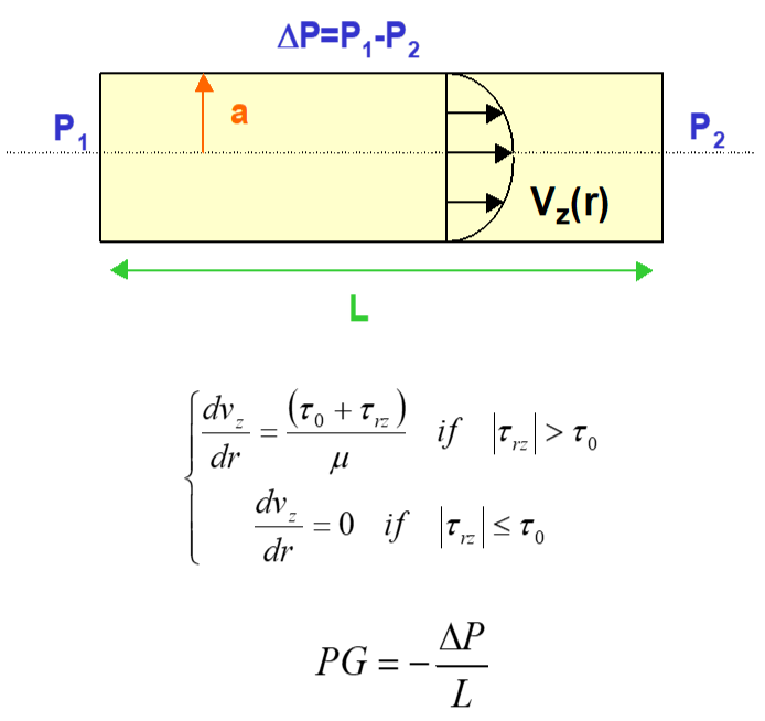
Calculation of shear stress using boundary condition:(0)=0
τ
rz
In[]:=
sol1=DSolve[D[r[r],{r,1}]PGr,[r],r]
τ
rz
τ
rz
Out[]=
[r]+
τ
rz
PGr
2
1
r
In[]:=
τ
rz
Out[]=
PGr
2
Calculation of velocity (r) between and using boundary condition: (a)=0
v
z
r=
-2
τ
0
PG
r=a
v
z
In[]:=
sol2=DSolve[D[[r],{r,1}]([r]+)/μ,[r],r]
v
z
τ
rz
τ
0
v
z
Out[]=
[r]++2r
v
z
1
PG
2
r
2
τ
0
2μ
In[]:=
v
z
PG
2
a
4μ
a
τ
0
μ
Out[]=
-PG-++2r
2
a
4μ
a
τ
0
μ
PG
2
r
2
τ
0
2μ
Calculation of Q1 flow rate between r= and r=a where velocity is given by (r)
-2
τ
0
PG
v
z
In[]:=
Q1=Integrate[2Pir[r],{r,-2/PG,a}]
v
z
τ
0
Out[]=
-PGπ-π+π+μ+
4
a
8μ
3
a
τ
0
3μ
2
a
2
τ
0
PGμ
4aπ
3
τ
0
2
PG
10π
4
τ
0
3μ
3
PG
Calculation of constant velocity between r=0 and r= using boundary condition: =(a)
v
0
-2
τ
0
PG
v
0
v
z
In[]:=
v
0
τ
0
τ
0
Out[]=
τ
0
2
τ
0
PG
μ
PG-+
2
a
4
2
τ
0
2
PG
4μ
Calculation of Q2 flow rate between r=0 and r= where velocity is constant equal to
-2
τ
0
PG
v
0
In[]:=
Q2=Integrate[2Pir,{r,0,-2/PG}]
v
0
τ
0
Out[]=
4π-a-+
2
τ
0
τ
0
2
τ
0
PG
μ
PG-+
2
a
4
2
τ
0
2
PG
4μ
2
PG
Total Flow Rate is equal to Q1+Q2
In[]:=
Q=Q1+Q2//Expand
Out[]=
-PGπ-π-
4
a
8μ
3
a
τ
0
3μ
2π
4
τ
0
3μ
3
PG
Volumetric Flow Rate for Pipe Flow of a Power Law Fluid
Q=nπ
3+
1
n
a
1
n
ΔP
2kL
1+3n
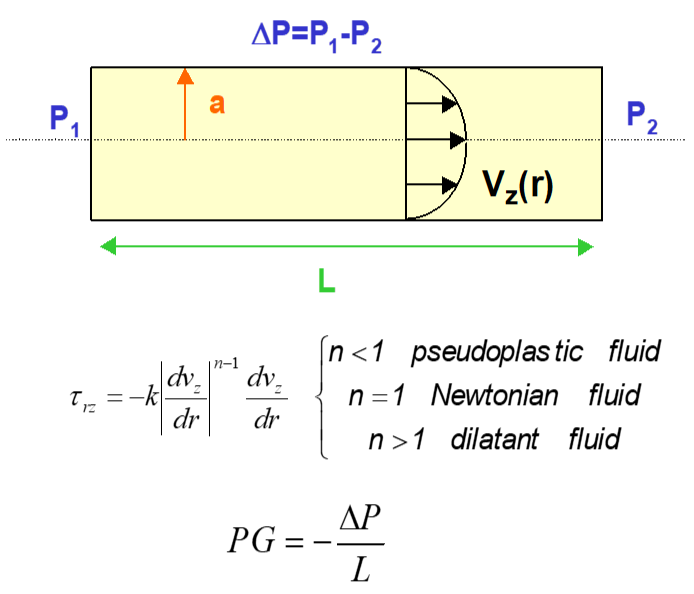
Clearing previous shear stress and velocity expressions
In[]:=
τ
rz
In[]:=
v
z
Calculation of shear stress using boundary condition:(0)=0
τ
rz
In[]:=
sol3=DSolve[D[r[r],{r,1}]PGr,[r],r]
τ
rz
τ
rz
Out[]=
[r]+
τ
rz
PGr
2
1
r
In[]:=
τ
rz
Out[]=
PGr
2
Calculation of velocity (r) between and using boundary condition: (a)=0
v
z
r=0
r=a
v
z
In[]:=
sol4=DSolve[D[[r],{r,1}]-(-[r]/k)^(1/n),[r],r]
v
z
τ
rz
v
z
Out[]=
[r]-r+
v
z
-1/n
2
1
n
-
PGr
k
1+
1
n
1
In[]:=
v
z
-1/n
2
1
n
-
PGa
k
1+n
Out[]=
-1/n
2
1
n
-
aPG
k
1+n
-1/n
2
1
n
-
PGr
k
1+
1
n
Calculation of Q flow rate between and where velocity is given by (r)
r=0
r=a
v
z
In[]:=
Q=Integrate[2Pir[r],{r,0,a}]//Simplify
v
z