Monitoring Trends in Burn Severity (MTBS): Data Analysis
by Mads Bahrami
by Mads Bahrami
My friends, Dr. Assaad Mrad, kindly informed me of Monitoring Trends in Burn Severity (MTBS) project. The main goal of this project is to “map the burn severity and extent of large fires across all lands of the United States from 1984 to present”. In this short computational essay, I have transformed MTBS Burned Areas Boundaries Dataset into computable dataset in Wolfram language.
One can get the raw data from the Burned Areas Boundaries Dataset . I have downloaded the zip file and put it in the same folder as this notebook.
In[]:=
data=Import[NotebookDirectory[]<>"mtbs_perimeter_data.zip","Data"];
Get the corresponding projection:
In[]:=
proj=Import[NotebookDirectory[]<>"mtbs_perimeter_data.zip","Projection"]/.("ReferenceModel"_)("ReferenceModel""NAD831986");
Dimensions
In[]:=
data//Dimensions
Out[]=
{1,4}
Looking at keys:
In[]:=
data〚1〛//Association//Keys
Out[]=
{LayerName,Geometry,Labels,LabeledData}
Looking at layer names:
In[]:=
Lookup["LayerName"][data]
Out[]=
{mtbs_perims_DD}
Looking at labels:
In[]:=
Lookup["Labels"][data]
Out[]=
{{Event_ID,irwinID,Incid_Name,Incid_Type,Map_ID,Map_Prog,Asmnt_Type,BurnBndAc,BurnBndLat,BurnBndLon,Ig_Date,Pre_ID,Post_ID,Perim_ID,dNBR_offst,dNBR_stdDv,NoData_T,IncGreen_T,Low_T,Mod_T,High_T,Comment}}
Create and association of list of association:
In[]:=
assoc=AssociationThread[Lookup["LayerName"]@data,#]&@Apply[Association,Transpose/@Apply[Thread[#1#2]&,MapAt[StringDelete["_"],Lookup["LabeledData"][data],{1,All,1}],{2}],{2}];
Create and association of list of association:
In[]:=
geometry=First/@(Map[<|"Geometry"#|>&,Lookup[{"Geometry"}]@data,{3}]//AssociationThread[Lookup["LayerName"]@data,#]&);
Join two associations and generate dataset for railroads:
In[]:=
ds=Dataset[Join@@@Transpose[Lookup["mtbs_perims_DD"][{assoc,geometry}]]][All,{"IgDate"(DateObject[Most[#],"Day"]&),"Geometry"(ReplaceAll[#,{FilledCurve[{{Line[pnts_]},__}]Polygon[GeoPosition@GeoGridPosition[pnts,proj]],Polygon[pnts_]Polygon[GeoPosition@GeoGridPosition[pnts,proj]]}]&)}];
Return length of dataset:
In[]:=
ds//Length
Out[]=
25614
Return column tags:
In[]:=
ds[1]//Keys//Normal
Out[]=
{EventID,irwinID,IncidName,IncidType,MapID,MapProg,AsmntType,BurnBndAc,BurnBndLat,BurnBndLon,IgDate,PreID,PostID,PerimID,dNBRoffst,dNBRstdDv,NoDataT,IncGreenT,LowT,ModT,HighT,Comment,Geometry}
A peak into dataset:
In[]:=
ds[;;2]
Out[]=

Data exploration
Data exploration
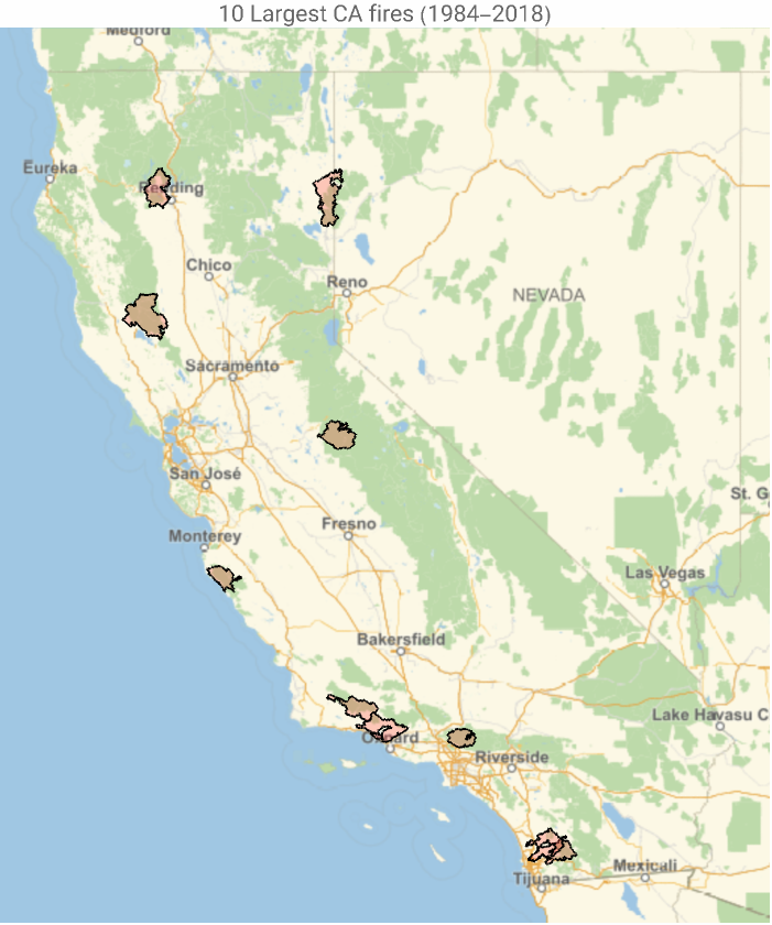
Obtain largest fires in CA in terms of burned area:
In[]:=
dt=Normal@ds[Select[StringContainsQ[#EventID,"CA"]&]][TakeLargestBy[#BurnBndAc&,10]][All,{Column[{#IncidName,DateString@#IgDate}],#Geometry}&];
Visualize the data (tooltip feature):
In[]:=
GeoGraphics{EdgeForm[Black],FaceForm[Red],Tooltip[#2,#1]&@@@dt},PlotLabel"10 Largest CA fires (1984-2018)",GeoRange
Out[]=
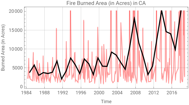
Return a time series of the fire-burned area in CA:
In[]:=
ts=ds[Select[StringContainsQ[#EventID,"CA"]&]][TimeSeries,{#IgDate,#BurnBndAc}&]
Out[]=
TimeSeries


Visualize it:
In[]:=
DateListPlotTimeSeriesAggregate[ts,],TimeSeriesAggregatets,,GridLinesAutomatic,AspectRatio12,FrameLabel{"Time","Burned Area (in Acres)"},FrameTicksAutomatic,DateRange{1984},{2018},,None,PlotStyle{Directive[Red,Opacity[.4]],Directive[Black,Thick]},PlotLabel"Fire Burned Area (in Acres) in CA",PlotLegends{"Monthly aggregate","Yearly aggregate"}
Out[]=


Return Thomas and Woolsey fires in CA:
In[]:=
dt2=ds[Select[StringContainsQ[#EventID,"CA"]&]][Select[MemberQ[{"THOMAS","WOOLSEY"},#IncidName]&]][All,{Column[{#IncidName,DateString@#IgDate,ToString[#BurnBndAc]<>" Arces"}],#Geometry}&];
Visualize it:
In[]:=
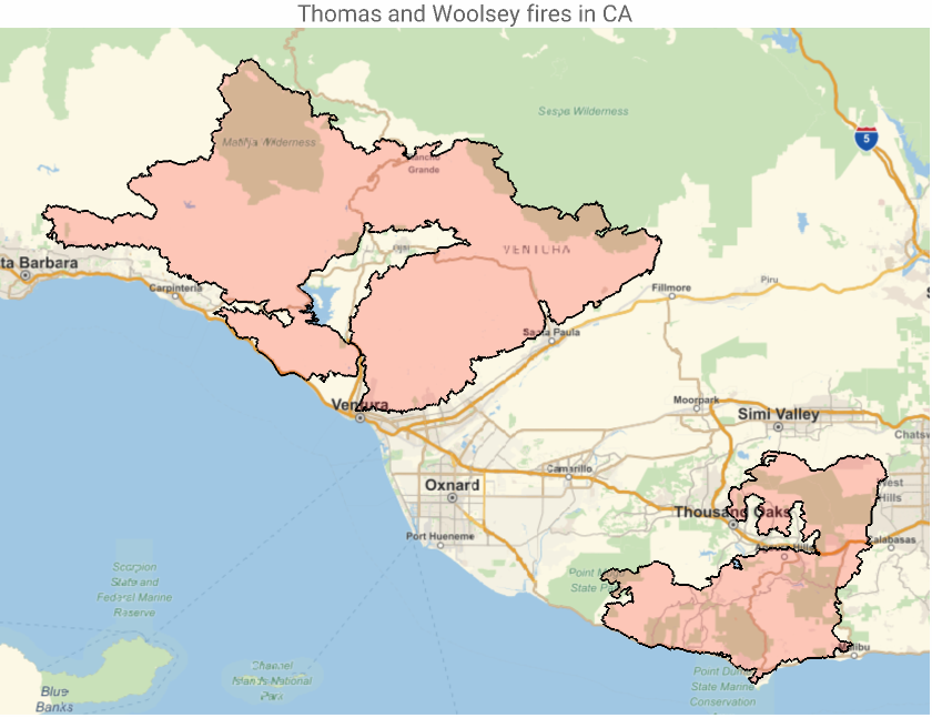
GeoGraphics[{EdgeForm[Black],FaceForm[Red],Tooltip[#2,#1]&@@@dt2},PlotLabel"Thomas and Woolsey fires in CA"]
Out[]=