Motivation: Biology, and especially computational molecular biology, has been growing exponentially for the last decade and perhaps even more. E.g. the problem of docking has always been crucial for drug design. Unfortunately common molecular dynamics approach to the problem often is too computationally expensive. It is even more relevant in the context of the ongoing COVID pandemic as we want to analyse enormous databases of bio-molecules in very short periods of time. One new approach to the problem suggests [1-3] using only surfaces of molecules because surfaces account for most of the factors impacting docking while their analysis requires vastly fewer computations.
Goal: To create a WL package for construction and visualization of protein surfaces. This can be the first step on the way to implementing auto-docking tools such as [1].
Results: The package implements the two main functions corresponding to the two types of surfaces. Tools necessary for sound work with proteins are also provided. All the code is packed into a package. The package has an installation function which runs automatically when it is imported.
Methods: More specifically the constructions of solvent accessible surface [4] (SAS) and of solvent excluded surface [4] (SES) are implemented using MSMS program [4]. The SAS of a protein is a surface formed by the points which a center of a probe solvent molecule rolling over the protein can occupy. The SES of a molecule is the boundary of the union of all possible probes that do not overlap with the protein. PDB files often do not have hydrogen atoms in them so one may want to protonate a protein before running surface analysis to gain a surface closer to the one acting in the real world. Often the impact of protonation on a surface is minimal, but it may not always be the case. A function for protonation is implemented using the Reduce program [5].
Future work: One possible direction the project can go is making use of the surfaces we now can construct. E.g. we can come up with some kind of overlap metric between protein surfaces and construct a cost function for how well two proteins fit in a given position. Having that we can run a 5D numerical optimization in space of relative positions of those two proteins and find the position in which they fit best. Having such an optimization tool we can run it through a database of docked pairs of proteins and find out its prediction accuracy. Furthering this approach we can compute different features of a surface such as charge density, hydropathy, curvature, etc. and train image-recognition-like CNNs to score certain regions of the surface to participate in an interface with another biomolecule.
I hope you are intrigued enough by the picture above so you are ready to read something about it. To understand the picture we first need to understand what exactly are the surfaces we want to construct.
Understanding SAS and SES
The following chapter is the shorten simplified narration of a part of the [4] article. The basic ideas of both types of surfaces are clear from the simple 2D picture:
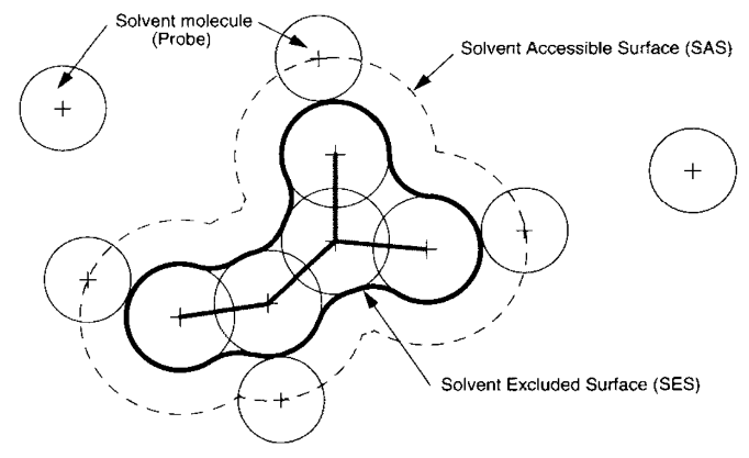
The solvent-accessible surface (SAS) is traced out by the center of the probe representing a solvent molecule. The solvent-excluded surface (SES) is the topological boundary of the union of all possible probes that do not overlap with the molecule.
Understanding what exactly we want to construct we can begin construction:
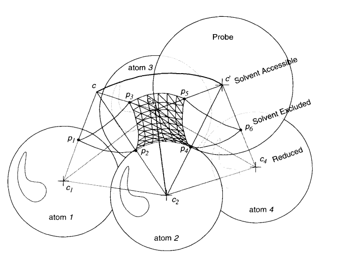
From a given fixed position c the probe can roll over pairs of atoms (here atoms 2 and 3).The geodesic arc (, ) sweeps out a part of a torus of axis (, ).The probe stops rolling over these two atoms when it hits a third atom (atom 4) that will define with atom 2 and 3 a new face (, , ) and a new spherical reentrant face (, ), for the SES.The center of the probe describes an arc of a circle (c, c’) that is an edge of the SAS.
p
2
p
3
c
2
c
3
c
2
c
4
c
3
p
4
p
6
p
5
Repeating the process of adding patches to the SAS and elements of torus and spheres to the SES we will get their complete representations. Complexity of the algorithm is O[N log(N)]. There do exist some technical problems, optimizations and nonobvious peculiarities. For the full description of the algorithm see the original article.
Visualisation of SAS
Now we understand the surfaces being constructed. To finally try something out by ourselves lets first import the package. If you are using Windows you need to install Cygwin before importing. Import looks like this:
In[]:=
CloudGet[CloudObject["https://www.wolframcloud.com/obj/polyachenko.yua/Published/ConstructPDBsurfaces.wl"]];
Lets pick a small protein for the demonstration:
In[]:=
pdbName="1aki";
First, we can just get the protein from the PDB database and see how does in look like in a standard secondary structure view:
In[]:=
pdb=DownloadPDB[pdbName];ImportString[pdb,"PDB"]
Out[]=

and then with the new implemented function we can get an understanding of how close to the protein can water molecules go:
In[]:=
DrawPDBSAS[pdb]
radii type: VanDerWaalsprobe radius = N,C,O,SN,C,O,S


Out[]=
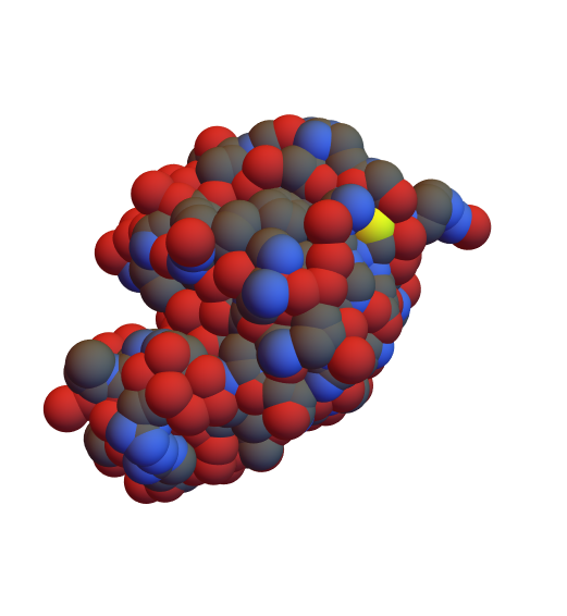
Here we can see a solvent accessible surface (SAS) of 1aki protein. Atoms are colored according to their chemical types. Atoms sizes are read from a WL database. Basic info is also printed to make the picture easier to interpret.
But this is not how the 1aki protein is in the real world. PDB files obtained from the X-ray experiments usually lack information about hydrogen positions. We can easily fix it:
In[]:=
pdbProtonated=ProtonatePDB[pdb];DrawPDBSAS[pdbProtonated]
radii type: VanDerWaalsprobe radius = N,C,O,H,SN,C,O,H,S

Out[]=
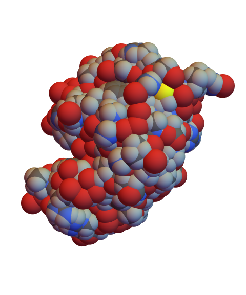
Protonation is performed via the Reduce program [5]. For now the the pH is assumed to be 7.0 and cannot be adjusted, but it is a clear possibility for the future development.
Before continuing to the SES surfaces we can play a bit with options here. E.g. probe radius for the ethanol would be , and we can see how this affects the SAS:
In[]:=
DrawPDBSAS[pdbProtonated,ProbeRQuantity[2.3,"Angstroms"]]
radii type: VanDerWaalsprobe radius = N,C,O,H,SN,C,O,H,S
Out[]=
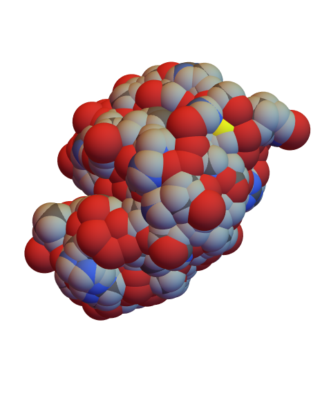
The main effect of the solvent change here is probably the closure of the gap in the left top corner, what can entail different consequences depending on your specific application of the data provided. Additionally sulfur atom became less exposed which can lead to the local shift in hydropathy and charge distribution what in its turn can affect docking process.
Another interesting experiment - we can see how exactly the molecule would look like if we could see it:
Finally, other types of radii to be visualized are available, e.g. covalent radii can give a glimpse on more low-level structure of smaller chemical compounds forming the protein:
Construction and visualization of SES
Solvent excluded surface (SES) of a protein is the best approximation of how the protein feels for the surrounding solvent. We can continue to work with the 1aki protein:
Unlike the SAS representation where we only had a 3D picture of the surface, here we have a full mathematical representation of the triangulated SES. The surface and triangulation were built by the MSMS program. According to its licence it can only be used for non-commercial studies. For commercial use one should install the MSMS package to get full licensing info.
Returning to protein surfaces, we can check everything we got out right here:
Returning to protein surfaces, we can check everything we got out right here:
E.g. vertices triangulation is built on look like:
The mesh itself is a list of triangles:
and meshInd are the indices of a corresponding vertices of polygons in vertices list:
Depending on your specific needs you can find balance between speed and accuracy of the surface. Here are two examples:
As we can see, the effect if hardly noticeable. It’s actually expected since the surface should be quite stable as long as a probe molecule can’t fall into the spaces between the atoms of the protein. This is not likely to happen because even the smallest real radius doesn’t diverge much:
so we can do what we want just for fun:
Bright future
Overall, the fact that these protein surfaces are now accessible in the Wolfram Language opens up a range of applications, enriching what can be done with their existing support for PDB integration and Protein entities. E.g. one can develop an algorithm to score the regions of the surface on how likely they are to participate in a bonding with a given ligand. This image was produced by the CNN trained on the 5 chemical and geometrical local features of the surface [1]:
Another application may embody the same idea but for the protein-protein docking [1]. The red area on the left picture is likely to be a part of a PP interface and blue area is not:
As you can see on the right diagram, using geometrical and chemical features of a surface enables one to efficiently distinguish the interface area of a surface.
Finally, having the fingerprints of each protein in a database, one can run a protein fitting based on the different kind of distances between fingerprints [1]:
It is absolutely clear that having the surface fingerprints one can find the position in which proteins are bound together.
Complete project work
Complete project work
Keywords
Keywords
◼
Computational biology
◼
Surfaces
◼
Protein
◼
PDB
◼
MeshRegion
◼
Import
Acknowledgment
Acknowledgment
John Cassel - Mentor
Krapp Lucien Fabrice, Matteo Dal Peraro - people at EPFL I work with on a project mentioned in the “future work” section.
Théo Beigbeder - WSS 2017 alumni. He told me about the school and motivated to participate for what I am deeply thankful.
References
References
◼
[1] Gainza, P., Sverrisson, F., Monti, F. et al. Deciphering interaction fingerprints from protein molecular surfaces using geometric deep learning. Nat Methods 17, 184–192 (2020).
doi.org/10.1038/s41592-019-0666-6
doi.org/10.1038/s41592-019-0666-6
◼
[2] Yoichi Murakami, Kenji Mizuguchi, Applying the Naïve Bayes classifier with kernel density estimation to the prediction of protein–protein interaction sites, Bioinformatics, Volume 26, Issue 15, 1 August 2010, Pages 1841–1848,
doi.org/10.1093/bioinformatics/btq302
doi.org/10.1093/bioinformatics/btq302
◼
[3] Porollo A, Meller J. Prediction-based fingerprints of protein-protein interactions. Proteins. 2007;66(3):630-645.
doi:10.1002/prot.21248
doi:10.1002/prot.21248
◼
[4] Word JM, Lovell SC, Richardson JS, Richardson DC. Asparagine and glutamine: using hydrogen atom contacts in the choice of side-chain amide orientation. J Mol Biol. 1999;285(4):1735-1747. doi:10.1006/jmbi.1998.2401
◼
[5] Sanner MF, Olson AJ, Spehner JC. Reduced surface: an efficient way to compute molecular surfaces. Biopolymers. 1996;38(3):305-320. doi:10.1002/(SICI)1097-0282(199603)38:3%3C305::AID-BIP4%3E3.0.CO;2-Y