CITE THIS NOTEBOOK: Low dimensionality to visualize the antibody–virus landscape for influenza by Tal Einav. Wolfram Community JAN 4 2023.
ORIGINAL ARTICLE: Einav, T., Creanga, A., Andrews, S.F. et al. Harnessing low dimensionality to visualize the antibody–virus landscape for influenza. NATURE Computational Science (2022). https://doi.org/10.1038/s43588-022-00375-1.
ORIGINAL ARTICLE: Einav, T., Creanga, A., Andrews, S.F. et al. Harnessing low dimensionality to visualize the antibody–virus landscape for influenza. NATURE Computational Science (2022). https://doi.org/10.1038/s43588-022-00375-1.
Article Abstract: Antibodies constitute a key line of defense against the diverse pathogens we encounter in our lives. Although the interactions between a single antibody and a single virus are routinely characterized in exquisite detail, the inherent tradeoffs between attributes such as potency and breadth remain unclear. Moreover, there is a wide gap between the discrete interactions of single antibodies and the collective behavior of antibody mixtures. Here we develop a form of antigenic cartography called a ‘neutralization landscape’ that visualizes and quantifies antibody–virus interactions for antibodies targeting the influenza hemagglutinin stem. This landscape transforms the potency–breadth tradeoff into a readily solvable geometry problem. With it, we decompose the collective neutralization from multiple antibodies to characterize the composition and functional properties of the stem antibodies within. Looking forward, this framework can leverage the serological assays routinely performed for influenza surveillance to analyze how an individual’s antibody repertoire evolves after vaccination or infection.
The following code reproduces the plots in the main text. Made on Mathematica version 13.0.0 for Windows. Sections can be opened by mouse click.
Raw data can be found in these initialization sections.
Figures
Figures
Figure 1: Neutralization Landscape for the HA Stem
Figure 1: Neutralization Landscape for the HA Stem
Constructing the Neutralization Landscape using monoclonal antibody neutralization data against a panel of influenza viruses.
Panel C: Neutralization Landscape
Panel C: Neutralization Landscape
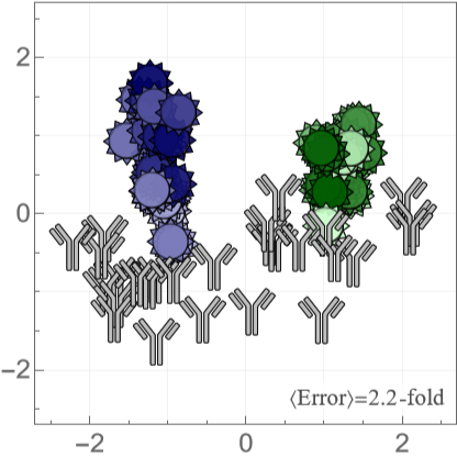
We use multidimensional scaling (MDS) to compute positions of antibodies and viruses, where an antibody-virus distance corresponds to the 50% inhibitory concentration =Molar. In the landscape below, placing the mouse above a virus or antibody will display its name.
d
IC
50
-10+d
10
The error at the bottom-right of the landscape shows the fold-error between the predicted (on the landscape) and measured for all antibody-virus pairs. We define (so that for each antibody-virus interactions) and average over all antibody-virus pairs with available measurements.
IC
50
IC
50
fold-error=
Max[Predicted,Measured]
IC
50
IC
50
Min[Predicted,Measured]
IC
50
IC
50
fold-error≥1
Some measurements lie outside the dynamic range of the experiment (> where =1.6·Molar=25). When both the and (i.e. the lower bound is satisfied), we exclude this measurement from the average fold-error to prevent artificially deflating the error. When the but , we define the fold-error as .
IC
50
max
IC
50
max
IC
50
-7
10
μg
mL
Measured>
IC
50
max
IC
50
Predicted>
IC
50
max
IC
50
Measured>
IC
50
max
IC
50
Predicted<
IC
50
max
IC
50
max
IC
50
Predicted
IC
50
In[]:=
createLandscape{coordsVirusStem,coordsAbStem},"Tooltip"True,"ErrorLabel""〈Error〉=","ErrorValue"landscapeError,"LabelColor"->

Out[]=
Panel D: Examples for an Antibody and Virus
Panel D: Examples for an Antibody and Virus
A deeper look into how one virus (H1N1 A/Michigan/45/2015) and one antibody (315-23-1C09) are positioned on the map. Each measurement is represented by a red circle with radius , and an antibody or virus must lie as close to all of these circles as possible. For clarity, we only show a small number of the measurements used to constrain their positions.
IC
50
r=Molar
log
10
IC
50
-10
10
In[]:=
Block{extraViruses={},virusOfInterest,antibodyOfInterest,coords,showEntries},(*Emphasizeavirusorantibody*)If[MemberQ[labelVirus,#],{virusOfInterest,antibodyOfInterest,coords}={#,None,coordsAbStem},{virusOfInterest,antibodyOfInterest,coords}={None,#,coordsVirusStem}];Show(*Showallentriesonlandscapewithsmallopacity*)createLandscape[{coordsVirusStem,coordsAbStem},"MarkerVirusOpacity"0.02,"MarkerAbOpacity"0.1],(*Entrieswhosesareshownasredcircles*)showEntries=CasesReplaceIf[virusOfInterest=!=None,Table[{antibody,data[virusOfInterest,antibody]},{antibody,labelAbStem}],Table[{virus,data[virus,antibodyOfInterest]},{virus,labelVirus}]],val:(_Real|_Integer):>Log10,,{2},{Switch[#,"H1N1 A/Michigan/45/2015","315-02-1H01"|"315-53-1A09"|"CR6261"|"CR9114"|"55-1D06","315-23-1C09","H1N1 A/Weiss/1943"|"H1N1 A/USSR/90/1977"|"H1N1 A/Beijing/262/1995"|"H1N1 A/California/07/2009"|"H1N1 A/Michigan/45/2015"|"H3N2 A/Colorado/2/1986"|"H3N2 A/Sichuan/2/1987"|"H3N2 A/Brisbane/10/2007"|"H3N2 A/Victoria/361/2011"|"H3N2 A/Singapore/INFIMH-160019/2016"],_};Graphics[{Opacity[0.3],{{Lighter[colorAbDecomposition,0.6],Thickness[0.0225],Circle[coords@#[[1]],#[[2]]]},{colorAbDecomposition,Thickness[0.0075],Circle[coords@#[[1]],#[[2]]]}}&/@showEntries}],createLandscape[If[virusOfInterest=!=None,{Association[],KeySelect[coordsAbStem,MatchQ[#,Alternatives@@First/@showEntries]&]},{KeySelect[coordsVirusStem,MatchQ[#,Alternatives@@Join[First/@showEntries,extraViruses]]&],Association[]}],"Tooltip"True],(*Antibodyorvirusofinterest*)If[virusOfInterest=!=None,ListPlot[{coordsVirusStem@virusOfInterest},PlotMarkersmarkerVirus[0.13,"OpacityFaceFormFactor"1],PlotStyleplotStyleVirus@virusOfInterest],ListPlot[{coordsAbStem@antibodyOfInterest},PlotMarkersmarkerAb[0.13],PlotStylecolorAbInMixture]],FrameTicksStyle22&/@{"H1N1 A/Michigan/45/2015","315-23-1C09"}
IC
50
val
-10
10
Out[]=
,
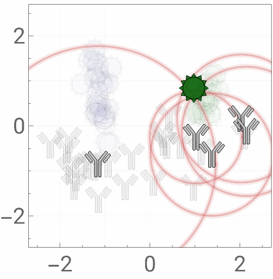
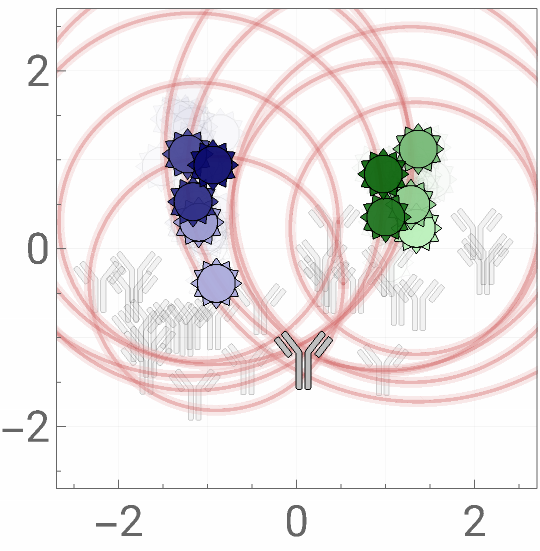
Figure 2: Quantifying the Spectrum of mAb Behavior
Figure 2: Quantifying the Spectrum of mAb Behavior
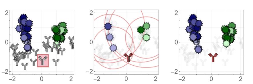
Once the positions of antibodies or viruses are determined on the landscape, additional entries can be rapidly added by using a few measurements to triangulate their coordinates and then predict their behavior against all other mapped entries. Currently, this implies that 6 antibody measurements can provide ~45 predictions; as the number of antibodies and viruses on the landscape grows, this predictive power will grow correspondingly.
In[]:=
resLeaveOneOutAntibody=;resLeaveMultiOutAntibody=;resLeaveOneOutVirus=;resLeaveMultiOutVirus=;
Canned: Leave-One-Out Analysis
Canned: Leave-One-Out Analysis
Panel A: Example of Triangulation
Panel A: Example of Triangulation
To test the predictive power of a new antibody not used for the MDS, we withhold one antibody from our dataset and recreate the landscape. On the new landscape, we triangulate the antibody using 6 neutralization measurements, and then predict the remaining 45 measurements.
◼
For visualization purposes, all landscapes are oriented as closely as possible to the Neutralization Landscape in Figure 1C (using translations, rotations, and reflections).
In[]:=
Block{coordsVirus,coordsAb,(*Antibodytowithhold*)leftOutAb="315-23-1C09",(*Virusesusedtotriangulatethewithheldantibody*)virusSubset={"H3N2 A/Brisbane/10/2007","H3N2 A/Sichuan/2/1987","H3N2 A/Colorado/2/1986","H1N1 A/Weiss/1943","H1N1 A/Michigan/45/2015","H1N1 A/Beijing/262/1995"},boxSize={0.37,0.42},plotRange=2.2{{-1,1},{-1,1}},frameTicksStyle=20},(*MDSresultsafterwithholdingantibody*){coordsVirus,coordsAb}=resLeaveOneOutAntibody[leftOutAb];(*Showtheoriginallandscapewiththewithheldantibodyboxed*)mapA=ShowcreateLandscape[{coordsVirusStem,Delete[coordsAbStem,Key[leftOutAb]]},"MarkerVirusSize"0.13,"MarkerVirusOpacity"1],GraphicsEdgeFormThickness[0.012],,FaceForm,Rectangle[coordsAbStem@leftOutAb-boxSize,coordsAbStem@leftOutAb+boxSize],ListPlot[{coordsAbStem@leftOutAb},PlotMarkersmarkerAb[0.15],PlotStylecolorAbInMixture],PlotRangeplotRange,FrameTicksStyleframeTicksStyle;(*Onthenewlandscape,triangulatethewithheldantibodyusing6measurements*)mapB=Show[triangulate[virusSubset,leftOutAb,{coordsVirus,coordsAb},"ShowMap"True]/.{(*Redcircles*)Opacity[0.8]Opacity[0.5]},PlotRangeplotRange,FrameTicksStyleframeTicksStyle];(*Wecannowpredicttheantibody'sinteractionwiththeremaining45viruses*)mapC=Show[createLandscape[{coordsVirus,coordsAb},"MarkerVirusSize"0.13,"MarkerVirusOpacity"1,"MarkerAbOpacity"0.05],ListPlot[{newCoord},PlotMarkersmarkerAb[0.15],PlotStylecolorAbDecomposition],PlotRangeplotRange,FrameTicksStyleframeTicksStyle];(*Plotting*)Grid[{{mapA,mapB,mapC}}]


Panel B: Summary Statistics for Ab Triangulation
Panel B: Summary Statistics for Ab Triangulation
This algorithm was carried out for all 27 stem antibodies, predicting 623 antibody-virus neutralization measurements.
Figure 4: Head+Stem Antibody Mixtures
Figure 4: Head+Stem Antibody Mixtures
By defining the range of all possible stem antibody behavior, we can also detect and computationally remove any non-stem behavior. In particular, we can create antibody mixtures containing both HA head and HA stem antibodies, and use their collective neutralization to characterize just the stem antibody within.
Panel C: Removing Head Neutralization
Panel C: Removing Head Neutralization
The right panel shows what happens when we computationally remove the head neutralization signal. The neutralization from all the blue H3N2 viruses are now given as lower bounds, since we correctly detected that the head antibody was causing their neutralization patterns. As a result, we can now predict the behavior of the stem antibody (red) and compare it to the true location of the stem antibody (gray, inferred from this antibody’s individual neutralization measurements that we did not access during the decomposition).
◼
We remove the head neutralization using measurements against the full H1N1 and H3N2 panel. For simplicity, we just show the resulting changes to a subset of viruses. (If we only considered this subset of measurements when removing the head neutralization, the results would have been slightly different, since we would not have as many virus pairs to constrain the neutralization measurements.)
Panel D: Two More Example Decompositions
Panel D: Two More Example Decompositions
We apply this decomposition to two additional mixtures containing (1 head + 1 stem, mixture #1) or (2 head + 1 stem, mixture #12).
Figure 5: Stem+Stem Antibody Mixtures
Figure 5: Stem+Stem Antibody Mixtures
Using the positions of each virus [Figure 1C], we can take a mixture’s neutralization data and infer the number of stem antibodies within as well as their stoichiometry and individual neutralization properties (i.e. their locations on these maps). We call this process a decomposition, since it takes the net neutralization of multiple antibodies and teases apart their individual behavior. We visualize the results by drawing the locations of the actual antibodies in the mixture in gray and the predicted antibodies from the decomposition in red.
Panel B: Predicted vs Measured Mixture IC50
Panel B: Predicted vs Measured Mixture IC50
We test how well the neutralization of each individual antibody predicts the combined neutralization of a mixture. We assume a competitive binding model, where all antibodies inhibit one another’s binding (i.e. no two antibodies can be simultaneously bound).
Panel C: Mixtures on the Landscape
Panel C: Mixtures on the Landscape
We can visualize the competitive binding model on our map by considering a mixture with two antibodies with a 50%/50% composition. We outline the regions inside which any virus will be ≥50% at different concentrations of antibody. Compared to each antibody’s individual neutralization (dashed circles), a mixture’s collective neutralization occurs over a larger region.
Panel D: Decomposing a Stem+Stem Mixture
Panel D: Decomposing a Stem+Stem Mixture
An example of the mixture #9 (stem+stem antibodies, true positions shown in gray) decomposed as two stem antibodies (red).
◼
Note that although the decomposition did not perfectly predict the positions of the antibodies nor their stoichiometry. However, both of these discrepancies somewhat offset each other, so that the neutralization profile is well-described by either the gray or red antibody mixture. In other words, this exemplifies that neutralization measurements may not uniquely identify an antibody mixture (especially when considering measurement error), and that multiple distinct antibody combinations could give rise to similar neutralization responses.
Panel E: Statistics for all Antibody Mixtures
Panel E: Statistics for all Antibody Mixtures
Analysis of all 14 antibody mixtures mixtures, stratified by the number of antibodies they contain. A monoclonal antibody is considered to be a "mixture" of 1 antibody.
Panel F: Two More Example Decompositions
Panel F: Two More Example Decompositions
Two additional examples where we decompose either a stem+stem mixture (#10) or a head+stem+stem mixture (#14).
Extra Figure: Neutralization Profiles (3D Visualization)
Extra Figure: Neutralization Profiles (3D Visualization)
A neat visualization tool to examine how the monoclonal antibodies and mixtures are decomposed using 1-3 antibodies.
Extra Figure: Removing Head Neutralization (3D Visualization)
Extra Figure: Removing Head Neutralization (3D Visualization)
Figure S1: Overview of MDS
Figure S1: Overview of MDS
We visualize the antibody-virus data and assess what fraction of the data is needed to make accurate predictions on withheld measurements.
Panel C: Schematic of Dataset
Panel C: Schematic of Dataset
Figure S5: Predicting Antibody Behavior in External Dataset
Figure S5: Predicting Antibody Behavior in External Dataset
Validating the maps and the ability to position and predict new mAb behavior using an external source of data [Nakamura 2013, Table 1]. We make the following substitutions to have a few extra predictions:
◼
ΔAA=2: H1N1 A/Brisbane/59/2007 H1N1 A/New York/08-1326/2008
◼
ΔAA=5: H3N2 A/Victoria/3/1975 H3N2 A/Bilthoven/1761/1976
Panel A: Triangulating New Antibodies using All Data
Panel A: Triangulating New Antibodies using All Data
Panel B: Predictions using a Subset of Data
Panel B: Predictions using a Subset of Data
Figure S6: Triangle Inequality
Figure S6: Triangle Inequality
For our bipartite data (where antibody-virus distance can be directly measured but not virus-virus or antibody-antibody distance), the typical triangle inequality is modified to the following form:
Interpretation of Virus-Virus Distance
Interpretation of Virus-Virus Distance
Figure S9: Decomposition Pathway
Figure S9: Decomposition Pathway
Here, we follow the decomposition algorithm for two mixtures: