Wolfram Cloud Document

Ask the Questions!

Can one hear the shape of a drum?

The phrase "Can one hear the shape of a drum?" is a famous question in mathematics and physics, originally proposed by Mark Kac in 1966. It refers to the problem of understanding whether different shapes can produce the same sound (or, more technically, have the same spectrum of vibrational frequencies).

The mathematical version of this problem involves eigenvalues of the Laplacian operator (which is related to the second derivative) and is a part of spectral geometry. The idea is to determine whether two different shapes (in this case, two-dimensional shapes like drumheads) can have the same set of Laplacian eigenvalues. These eigenvalues correspond to the frequencies of vibration (or "tones") of the drum.

For a long time, it was unknown whether the shape of a drum could be uniquely determined by its sound. However, in 1992, Carolyn S. Gordon, David L. Webb, and Scott Wolpert demonstrated that different shapes can indeed have the same set of vibrational frequencies. So, strictly speaking, one cannot always hear the shape of a drum.

That being said, there are many restrictions and special cases where the shape can indeed be inferred from the sound, and this remains an active area of research in both mathematics and physics.

For a more detailed and technical explanation, you might want to refer to some textbooks or scientific papers on spectral geometry or wave equations.

Given a polygonal region how do I compute the eigensystem?

Computing the eigensystem for a polygonal region in the context of the "drum problem" essentially involves solving the Helmholtz equation, which is a partial differential equation. The Wolfram Language has built-in functionality to solve such equations, and therefore to compute the eigensystem for a given region.Here's a simple example to illustrate how you could do this for a square region. This example finds the first 6 eigenvalues and eigenfunctions for a unit square:

region=Rectangle[{0,0},{1,1}];{n,vals,funs}=NDEigensystem[{-Laplacian[u[x,y],{x,y}],DirichletCondition[u[x,y]==0,True]},u[x,y],{x,y}∈region,6];vals

Insert and evaluate

Insert

Copy

In this code,

NDEigensystem

is the function that computes the eigenvalues and eigenfunctions. The first argument to

NDEigensystem

is the operator (in this case, the negative Laplacian, which represents the vibration of the drumhead), and the second argument is the function we're solving for (

u[x,y]

). The third argument specifies the region over which we're solving the equation (

{x,y}∈region

), and the fourth argument is the number of eigenvalues and eigenfunctions to find (

).The output of this code will be the first 6 eigenvalues of the Laplacian on the unit square, which represent the frequencies of the first 6 modes of vibration of the drumhead. The funs list will contain the corresponding eigenfunctions, which represent the shapes of these modes of vibration.Please note that this is a relatively complex topic, and understanding the output of this code requires some background in partial differential equations and spectral theory.

Polyabolo Configurations

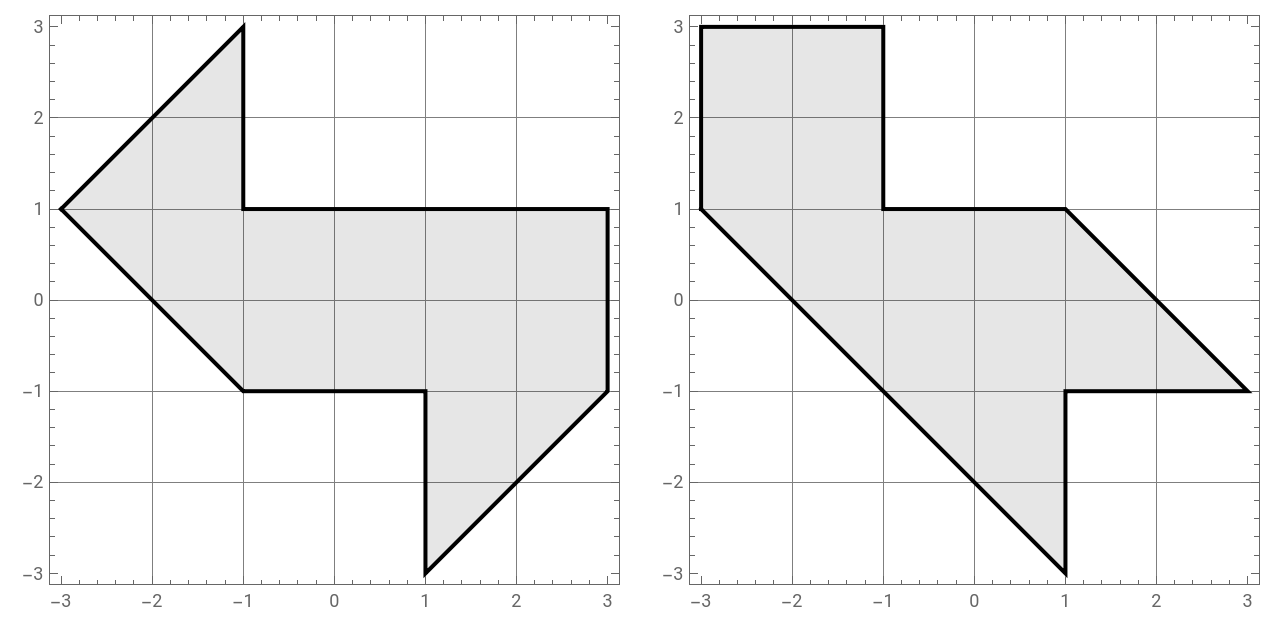
A simple example of isospectral manifolds is the pair of polyabolo configurations known as bilby and hawk (see MathWorld):

In[]:=

bilby=Polygon[{{-3,1},{-1,-1},{1,-1},{1,-3},{3,-1},{3,1},{1,1},{-1,1},{-1,3}}]

Out[]=

Polygon

Number of points: 9

Embedding dimension: 2



In[]:=

hawk=Polygon[{{-3,1},{-1,-1},{1,-3},{1,-1},{3,-1},{1,1},{-1,1},{-1,3},{-3,3}}]

Out[]=

Polygon

Number of points: 9

Embedding dimension: 2



In[]:=

GraphicsRow[{Graphics[{EdgeForm[{Thick,Black}],Opacity[0.1],bilby},FrameTrue,GridLinesAutomatic],Graphics[{EdgeForm[{Thick,Black}],Opacity[0.1],hawk},FrameTrue,GridLinesAutomatic]}]

Out[]=

Eigensystem

For the 2D Helmholtz problem specify the Laplacian operator with homogeneous Dirichlet boundary conditions

In[]:=

{ℒ,ℬ}=-

∇

{x,y}

u[x,y],DirichletCondition[u[x,y]0,True];

Compute the 9 smallest eigenvalues and eigenfunctions of the Helmholtz problem for each polygonal region:

In[]:=

{eigenvalues[1],eigenfunctions[1]}=NDEigensystem[{ℒ,ℬ},u,{x,y}∈bilby,9]

In[]:=

{eigenvalues[2],eigenfunctions[2]}=NDEigensystem[{ℒ,ℬ},u,{x,y}∈hawk,9]

In[]:=

Dataset@AssociationThread[Range[9],Transpose@{eigenvalues[1],eigenvalues[2],-Round@Log[10,Abs[eigenvalues[1]-eigenvalues[2]]]}]

Out[]=

1	2.54626	2.54754	3
2	3.66551	3.66549	5
3	5.19549	5.19549	6
4	6.54861	6.54919	3
5	7.26944	7.27151	3
6	9.23097	9.23376	3
7	10.6265	10.6346	2
8	11.5747	11.5751	3
9	12.3728	12.3739	3

Visualization

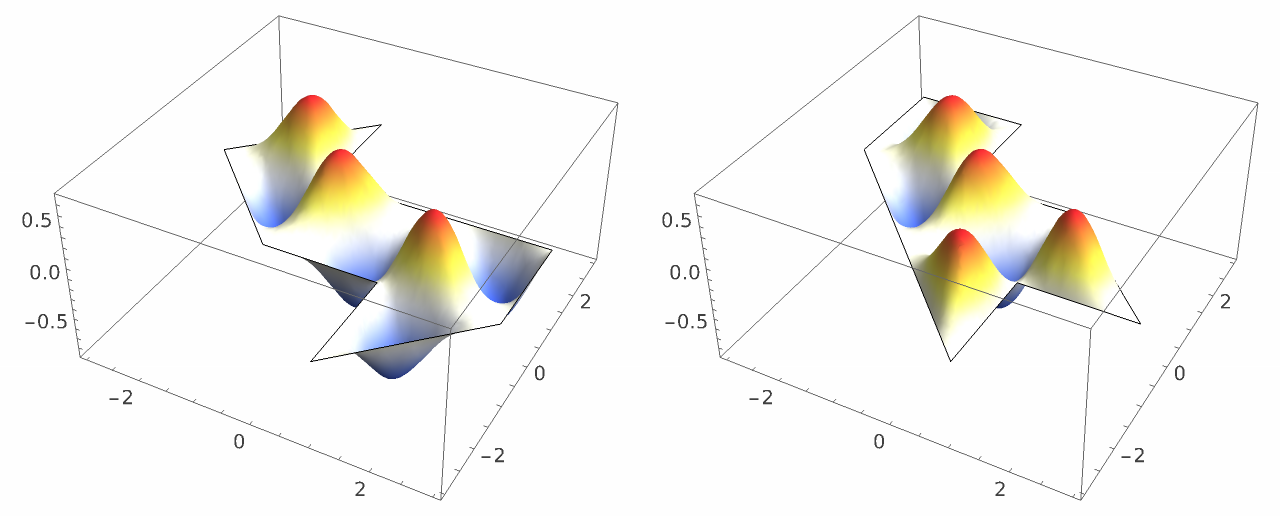
Plot the (squared) eigenfunctions for the lowest 9 eigenvalues for each polygonal region using TabView:

Out[]=

Higher Precision Solutions

According to Toby Driscoll:

A little-known method due to Descloux and Tolley performs far better than all of these. The underlying principle is to exploit the well-known expansions of an eigenfunction near the corners. The criterion that selects eigenvalues is the matching of values and normal derivatives of the local expansions at interfaces within the polygons.

In[]:=

method=Iconize[Method{"PDEDiscretization"{"FiniteElement","MeshOptions"{"MaxCellMeasure"0.001}}},"Method"]

Out[]=

Method

In[]:=

{eigenvalues[1],eigenfunctions[1]}=NDEigensystem{ℒ,ℬ},u,{x,y}∈bilby,10,

Method

;

In[]:=

{eigenvalues[2],eigenfunctions[2]}=NDEigensystem{ℒ,ℬ},u,{x,y}∈hawk,10,

Method

;

These eigenvalues agree to at least 4 decimal places but do not agree to this precision to the values obtained by Driscoll (he computed 25 eigenvalues and modes for each polygon to about 12 digits of accuracy):

In[]:=

Dataset@AssociationThread[Range[10],Transpose@{eigenvalues[1],eigenvalues[2],-Round@Log[10,Abs[eigenvalues[1]-eigenvalues[2]]]}]

Out[]=

1	2.53839	2.53839	5
2	3.65594	3.65595	5
3	5.17642	5.17643	5
4	6.53774	6.53773	5
5	7.2489	7.24891	5
6	9.20967	9.20969	5
7	10.5975	10.5975	5
8	11.5415	11.5415	5
9	12.337	12.337	11
10	13.055	13.055	4

Toby Driscoll hypothesizes that the accelerated convergence for the 9th eigenvalues occurs because the symmetries of these eigenfunctions about the corners cause many of the Fourier coeﬃcients to be exactly zero.

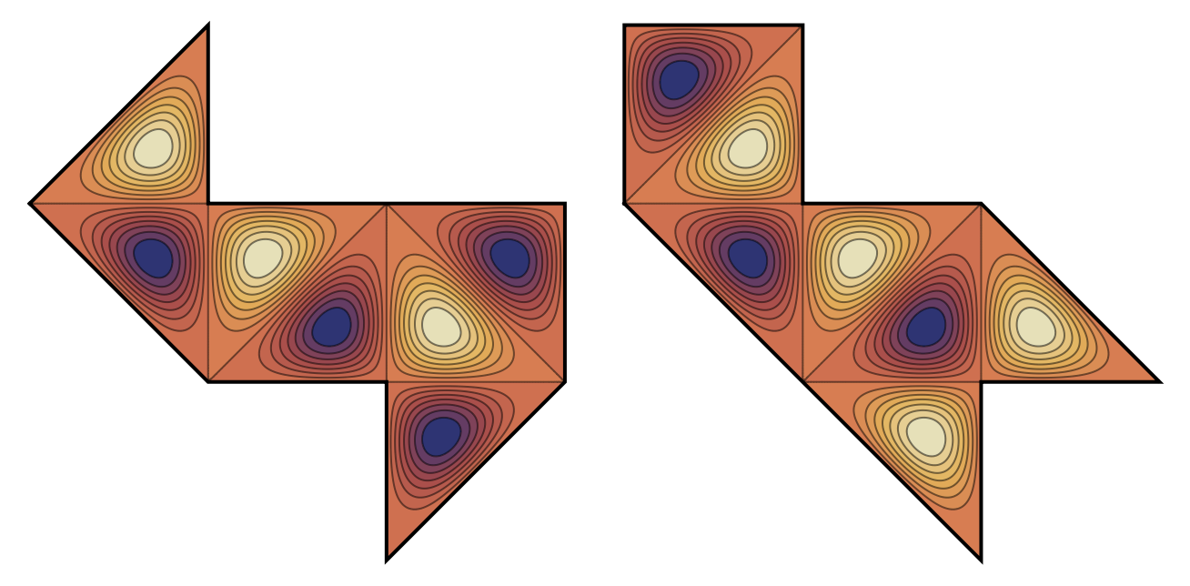
ContourPlot of the eigenfunctions for the

eigenvalue for each polygonal region:

Out[]=