Deciding where to live is one of the most important choices we make, as it impacts our finances and overall quality of life. This project aims to help people find the best places to live based on their income, living costs, and commuting expenses. We started by looking at a fixed case of three cities in Texas—Dallas, Plano, and Fort Worth—to see which offers the best value for those working in Dallas. By comparing living and travel costs, we identified which city allows for the most savings and a better lifestyle. As the project evolved, we expanded our approach to cover the entire United States. This new, working and flexible model helps people across the US find the ideal balance between where they live and work, ensuring they can make the most of their earnings and maximise their savings. This research not only help individuals in making smarter living choices but also contributes to broader conversations about economic mobility and urban planning.
Introduction
Introduction
For many people their place of residence and place of work differ due to the differences in housing prices and other economic factors. Sometimes, people find it hard to find the optimal place in which to live according to the factors they consider. Furthermore, there might be some other costs that are not considered in the living indices for the city that one is planning to reside in, such as travel costs if the place in which they work is far. Thus, considering all these factors, people’s residence choice relies significantly on their desire to maximize their savings. Hence, we constructed this project for people to find the best optimal place to live according to their income.
Towards this objective, we started with a fixed case of one “default” city and two “alternative” cities. Firstly, we look at Dallas, Texas as the city in which the individual works and is considering living as well. Then, we look at two alternative cities also within Texas, Plano and Fort Worth, respectively, as relative substitutes for the individual’s residence choice. After completing the analysis for this fixed scenario, we code a cityOptimizer function which enables the same analysis but for any three cities and individual yearly salary inputs to examine the choice in other locations within the United States. It is important to note that, travel costs are measured only between cities and not within cities. This is because within-city travel costs are measured by the data retrieved through Wolfram Alpha (The Council For Community And Economic Research, 2024).
Cost of Living Index: Fixed Case
Cost of Living Index: Fixed Case
Entity Creator Function
Entity Creator Function
This code defines a function called entityCreator that creates an entity based on a given city name. The function takes a string input and uses the WolframAlpha function to query Wolfram Alpha for the city. The result of the query is then returned as the entity of the city. This function is being used to simplify the process of generating city entities from city names and making it easier to work with city-specific data in subsequent computations, especially for geographical visualisations.
In[]:=
entityCreator[cityString_String]:=WolframAlpha[cityString,"Result"]
Creating City Entities
Creating City Entities
This code creates a list called entityCities that includes Dallas, Plano, and Fort Worth in Texas. Subsequently, it will help further in managing and analyzing data for the cities all at once.
Using the entityCreator function, it identifies these cities and makes them into entities.
In[]:=
entityCities={entityCreator["Dallas, Texas"],entityCreator["Plano, Texas"],entityCreator["Fort Worth, Texas"]}
Out[]=
,,
Retrieving Cost of Living Indices for Cities
Retrieving Cost of Living Indices for Cities
This code creates a list called livingIndices that includes the cost of living indices for Dallas, Plano, and Fort Worth, Texas. It uses WolframAlpha to look up the living cost index for each city, and then extracting the result. This way, it is easy to compare the cost of living in these cities, further helping in making decisions about where living expenses might be higher or lower.
In[]:=
livingIndices={WolframAlpha["living cost index in Dallas, Texas","Result"],WolframAlpha["living cost index in Plano, Texas","Result"],WolframAlpha["living cost index in Fort Worth, Texas","Result"]}
Out[]=
{102.2,113.3,94.2}
Baseline Value for Comparing your Salary
Baseline Value for Comparing your Salary
baseLineMoney is the median value taken from “The council for community and economic research” after comparing the maximum and minimum monthly expenses in the US. This is the amount of money used to compare the per person’s salary to
In[]:=
baseLineMoney=7500;
Travel Cost Index Calculation
Travel Cost Index Calculation
To determine a travel cost index, this code defines a function named calculateTravelIndex. This travel cost index helps standardize travel expenses relative to the baseline monetary value given above.
This function takes the travel cost t as input and uses the formula shown below. After getting the final result, it is rounded to two decimal places using the Round function.
In[]:=
calculateTravelIndex[t_]:=Round[(40*t)/baseLineMoney*100,0.01];
Calculating Plano and Fort Worth’s Travel and Living Cost Index
Calculating Plano and Fort Worth’s Travel and Living Cost Index
The costsOfTravel list takes out the travel expenses for driving between cities in Texas. The first value is 0, indicating no travel cost as the first condition states that the person is working in Dallas and staying in Dallas. The second value calculates the cost of driving from Plano to Dallas. It takes the average gas price in Plano, divides it by the car’s fuel efficiency (28 miles per gallon), and multiplies by the distance between the two cities. Similarly, the third value calculates the cost of driving from Fort Worth to Dallas using the average gas price in Fort Worth and the distance between Fort Worth and Dallas. This helps in compare travel costs from Plano and Fort Worth to Dallas, Texas.
In[]:=
costsOfTravel=0,*QuantityMagnitude@TravelDistance[{entityCities[[2]],entityCities[[1]]}],*QuantityMagnitude@TravelDistance[{entityCities[[3]],entityCities[[1]]}]
QuantityMagnitude@WolframAlpha["average gas price in Plano, Texas",{{"Result",1},"ComputableData"}]
28
QuantityMagnitude@WolframAlpha["average gas price in Fort Worth, Texas",{{"Result",1},"ComputableData"}]
28
Out[]=
{0,2.40189,4.12345}
The travelIndices list calculates travel cost indices for trips from Plano to Dallas, Texas and from Fort Worth to Dallas, Texas. Again, the first value is 0, indicating no travel cost as it is considering the fixed case. The second and third values apply the calculateTravelIndex function to the travel costs from Plano and Fort Worth to Dallas, converting these costs into travel indices for comparison.
In[]:=
travelIndices={0,calculateTravelIndex[costsOfTravel[[2]]],calculateTravelIndex[costsOfTravel[[3]]]}
Out[]=
{0,1.28,2.2}
Table creates a list called totalLivingIndices by adding the results of livingIndices and travelIndices for each of the three cities. This combines the cost of living with travel costs, and providing a index for comparing overall expenses in Dallas, Plano, and Fort Worth.
In[]:=
totalLivingIndices=Table[livingIndices[[i]]+travelIndices[[i]],{i,1,3}]
Out[]=
{102.2,114.58,96.4}
Visual Output Representations
Visual Output Representations
Geographical Cost Index Map
Geographical Cost Index Map
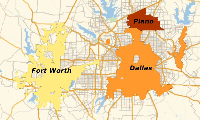
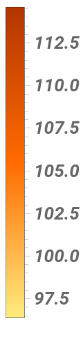
resultsMap generates a geographic plot that visually represents living cost indices for three Texas cities. It pairs each city with its the total living index taken out previously and later plots these values on the geoRegionValuePlot.
In[]:=
resultsMap=GeoRegionValuePlot[Thread[{entityCities[[1]],entityCities[[2]],entityCities[[3]]}->{totalLivingIndices[[1]],totalLivingIndices[[2]],totalLivingIndices[[3]]}],GeoLabels->True,ImageSize->400,LabelStyle->{13,Bold,Italic}]
Out[]=
Index of Costs Comparison Grid
Index of Costs Comparison Grid
resultIndexGrid constructs a grid that represents cost indices for Dallas, Plano, and Fort Worth, Texas. It has a header row that labels each city and organizes the data into three categories: “Living,” “Travel,” and “Total” costs. Each row under these categories shows the respective index values for each city, which further help in better analysing and getting a clear comparison of the costs.
In[]:=
resultIndexGrid=Grid[{{Style["Index of Costs",Bold,FontFamily->"Times New Roman",FontSize->14],Style["Dallas, Texas",Bold,FontFamily->"Times New Roman",FontSize->14],Style["Plano, Texas",Bold,FontFamily->"Times New Roman",FontSize->14],Style["Fort Worth, Texas",Bold,FontFamily->"Times New Roman",FontSize->14]},{Style["Living",FontFamily->"Arial"],Style[livingIndices[[1]]],Style[livingIndices[[2]]],Style[livingIndices[[3]]]},{Style["Travel",FontFamily->"Arial"],Style[travelIndices[[1]]],Style[travelIndices[[2]]],Style[travelIndices[[3]]]},{Style["Total",FontFamily->"Arial"],Style[totalLivingIndices[[1]]],Style[totalLivingIndices[[2]]],Style[totalLivingIndices[[3]]]}},Frame->All]
Out[]=
Index of Costs | Dallas, Texas | Plano, Texas | Fort Worth, Texas |
Living | 102.2 | 113.3 | 94.2 |
Travel | 0 | 1.28 | 2.2 |
Total | 102.2 | 114.58 | 96.4 |
Salary
Salary
The representative salary is an estimated salary for a household taken from “pay scale” for Dallas, Texas.
Use representativeSalary to input any salary per person in numeric value.
representativeSalary=100000;
The function convertToMonetaryTerms takes a cost index and converts it to monetary terms. This conversion makes it easier to understand the cost index in terms of actual currency, making it better to interpret and compare the costs.
This function provides the result by multiplying the index by a baseline monetary value (baseLineMoney) and then dividing by 100.
In[]:=
convertToMoneraryTerms[givenIndex_]:=;
baseLineMoney*givenIndex
100
Table converts cost indices for living, travel, and total living expenses into monetary terms using the convertToMonetaryTerms function. It creates three lists: livingMoneyTerms, travelMoneyTerms, and totalLivingMoneyTerms. Each of the lists are generated by applying the function to the indices for the three cities (Dallas, Plano, and Fort Worth). By repeating over the indices with a loop, the code translates the percentage-based indices into monetary amounts.
In[]:=
livingMoneyTerms=Table[convertToMoneraryTerms[livingIndices[[i]]],{i,1,3}];travelMoneyTerms=Table[convertToMoneraryTerms[travelIndices[[i]]],{i,1,3}];totalLivingMoneyTerms=Table[convertToMoneraryTerms[totalLivingIndices[[i]]],{i,1,3}];
The calculateNetIncome function determines the net monthly income by subtracting monthly expenses from a person’s monthly salary. It takes the annual salary, divides it by 12 to get monthly earnings, and then subtracts the specified expenses.
calculateNetIncome[moneyTerms_]:=-moneyTerms;
representativeSalary
12
The given code creates a list named netIncome by calculating the net income for each element in the list totalLivingMoneyTerms. It does this by applying the function calculateNetIncome to each element in the variable totalLivingMoneyTerms taken out previously.
In[]:=
netIncome=Table[calculateNetIncome[totalLivingMoneyTerms[[i]]],{i,1,3}];
The code constructs a grid, netIncomeGrid, which organizes and displays financial data for Dallas, Plano, and Fort Worth, Texas. The rows contain the “Living,” “Travel,” “Total,” and “Net Income” costs. Each cost category displays the values from the lists livingMoneyTerms, travelMoneyTerms, totalLivingMoneyTerms, and netIncome.
In[]:=
netIncomeGrid=Grid[{{Style["Costs",Bold,FontFamily->"Times New Roman",FontSize->14],Style["Dallas, Texas",Bold,FontFamily->"Times New Roman",FontSize->14],Style["Plano, Texas",Bold,FontFamily->"Times New Roman",FontSize->14],Style["Fort Worth, Texas",Bold,FontFamily->"Times New Roman",FontSize->14]},{Style["Living",FontFamily->"Arial"],Style[livingMoneyTerms[[1]]],Style[livingMoneyTerms[[2]]],Style[livingMoneyTerms[[3]]]},{Style["Travel",FontFamily->"Arial"],Style[travelMoneyTerms[[1]]],Style[travelMoneyTerms[[2]]],Style[travelMoneyTerms[[3]]]},{Style["Total",FontFamily->"Arial"],Style[totalLivingMoneyTerms[[1]]],Style[totalLivingMoneyTerms[[2]]],Style[totalLivingMoneyTerms[[3]]]},{Style["Net Income",FontFamily->"Arial"],Style[netIncome[[1]]],Style[netIncome[[2]]],Style[netIncome[[3]]]}},Frame->All]
Displaying Standardized Monthly Living Costs in the US
Displaying Standardized Monthly Living Costs in the US
The variable totalUSIndex contains a text label and a variable called baseLineMoney. This is defined within the code to display the baseline monetary value for comparison.The Row function combines the string “US standardized monthly living costs ($) = “ with the value of baseLineMoney. When executed it creates a labeled display of the standardized monthly living costs in the US, where the baseLineMoney shows the monetary value defining the costs.
Use the variable totalUSIndex to find out the standardized monthly living costs in dollars.
Highest Net Income City Analysis
Highest Net Income City Analysis
The code evaluates which of the three cities from Plano, Fort Worth and Dallas offer the highest net income by comparing their indices in totalLivingIndices. Using the Which function, it checks conditions to identify the city with the lowest index value. After it is evaluated, it displays a column containing a message indicating the city where net income is maximized, and further followed by visual elements like resultsMap, totalUSIndex, resultIndexGrid, and netIncomeGrid.
To use the function you have to define the cost of living indices for the cities of your choice the same way it is defined for Fort Worth,Frisco and Dallas, along with additional data. Evaluate the `Which` function to compare these indices and display the city with the highest net income. The output will provide a message about which city can make you maximize your income and show visual such as maps, indexes, and grids.
Final Visual Output
Final Visual Output
Determining Cost of Living Data Availability
Determining Cost of Living Data Availability
The function testWhetherThereIsData, defined in the code, uses Wolfram Alpha to determine whether a city’s cost of living index is available. The function takes a city name as a string. It starts by querying Wolfram Alpha for the cost of living index for the given city. The result is then checked to determine if it is a numerical value. Based on this check, the function generates a styled message saying if the code is available or not.
To use the function testWhetherThereIsData[“CityName”], the input is a string called “CityName”which needs to be replaced with the name of the city you want to check the living cost of index for.
For instance while checking for “Dallas, Texas”, Wolfram Alpha finds the data in its data base so the message “There is data! :D” is shown in green.
However, while checking for “Pacifica, California”, Wolfram Alpha could not find the data so the result displayed “No data available on this city. Please try another one. :(“
Now, having defined the fixed case in its entirety, the cityOptimizer function can now be defined, following the fixed case structure but for four variable inputs:
1
.defaultCity: the name and state, in string form, of the city in which the individual will work and is considering living too.
For instance, “Dallas, Texas”.
2
.alternative1City: the name and state, in string form, of the first alternative city in which the individual is considering living.
For instance, “Plano, Texas”.
3
.alternative2City: the name and state, in string form, of the second alternative city in which the individual is considering living.
For instance, “Fort Worth, Texas”.
4
.salary_: the individual’s yearly salary as a real positive number.
For instance, 100000.
The following is an example you can run to produce the same output as in the previously explored fixed case.
Now, this is an example with different city and salary inputs.
Conclusion
Conclusion
To conclude, in our project, we navigated the challenge of choosing the best place to live based on socioeconomic factors like living and cross-city travel costs. We focused on Texas, specifically Dallas, Plano, and Fort Worth as examples to show how comparing living costs and travel expenses can help individuals make smart residential decisions. Then, the cityOptimizer function was effectively created, prior to which the testWhetherThereIsData function should be evaluated by the individual for the three options which they are considering. Otherwise, cityOptimizer will not run properly.
As a result, in the Texan case, it was seen that Fort Worth is a more cost-effective city than both Dallas and Plano. Hence, an individual would maximize their net income by living in Fort Worth even if they are working in Dallas. However, in the Californian case, San Francisco is a better choice than Cupertino or San Jose to maximize net income. Therefore, an individual would find it best to work and live in San Francisco.
Future Directions
Future Directions
Even though we had a limited time to work on the project, we wanted to give it future enhancements such as extensions to the code by considering more economic and general factors such as availability and quality of nearby schools, airports, hospitals, etc. In turn, these could be assigned importance weights by the individual such that they can model their preferences more accurately and get a more specialised result to their case. We would like for it to extend to other parts for the world as well so it is more flexible and accessible to people all over the world. We would also like to consider even more alternative cities. Finally, to make the results more specific and give the exact location for people to live we would like to include a function that generates the zip codes or communities that the person should live in.
Acknowledgements
Acknowledgements
I would like to acknowledge my mentor, Carlos Angulo, for helping me through every step of my project, being very patient with me and reviewing my work at every step so there are no major mistakes in the code and the essay. I would also like to thank the TAs Nora Popescu and Alisa Zaitseva to helping me develop my code step by step and helping me with the structure to my project. Without my mentor and the TAs this project and camp would have not been as amazing as it was.
Bibliography
Bibliography
◼
The Council For Community And Economic Research, 2024. http://c2c.coli.org/compare.asp?action=sample. Accessed 11 July 2024.
◼
Payscale, 2024. Average Salary in Dallas, Texas, www.payscale.com/research/US/Location=Dallas-TX/Salary. Accessed 11 July 2024.
◼
CITE THIS NOTEBOOK
CITE THIS NOTEBOOK
Optimize best living locations based on cost of living and potential income
by Mannat Dhillon
Wolfram Community, STAFF PICKS, July 12, 2024
https://community.wolfram.com/groups/-/m/t/3217049
by Mannat Dhillon
Wolfram Community, STAFF PICKS, July 12, 2024
https://community.wolfram.com/groups/-/m/t/3217049