Estimation of NRTL Parameters and Common-Tangent Continuation for Liquid–Liquid Equilibrium in the Water + 5-HMF + 1-Butanol System
Housam Binous and Abdelmalek Hasseine
Housam Binous and Abdelmalek Hasseine
This notebook presents a computational thermodynamics study of the ternary liquid–liquid equilibrium (LLE) system composed of water, 5-hydroxymethylfurfural (5-HMF), and 1-butanol — a system of practical interest for biomass-derived furanic compound extraction. The authors use experimental tie-line data (given in weight percent and converted to mole fractions using the molecular weights of the three components) collected at three temperatures: 313.15 K, 323.15 K, and 333.15 K, each set consisting of coexisting organic-phase and aqueous-phase compositions.
The first major part of the analysis (Part A) focuses on regressing NRTL (Non-Random Two-Liquid) activity coefficient model parameters from the experimental tie lines. Rather than relying on a single local optimizer, we implement a hybrid strategy: a Particle Swarm Optimization (PSO) algorithm first performs a global search over the six unknown NRTL binary interaction parameters, minimizing a least-squares objective function that measures the mismatch between calculated and experimental phase compositions (enforced via iso-activity equality constraints solved with FindRoot for each tie line).
Once PSO converges to a good starting point, the solution is refined using a local Interior Point method (via FindMinimum), yielding a marginal improvement in the objective function and a final RMSD around 0.0025 for the composition fit at 313.15 K. The resulting NRTL interaction parameter matrix and the fixed non-randomness parameters (α = 0.2 for each binary pair) are then used to reconstruct the τ and G matrices needed for subsequent thermodynamic calculations.
Part B shifts to computing the full binodal (solubility) curve and tie lines using a geometric equilibrium criterion rather than direct algebraic solving: the common tangent plane construction on the molar Gibbs energy of mixing surface. The equal-activity/equal-chemical-potential conditions between the two coexisting phases are expressed as a system of nonlinear equations (common tangent line conditions plus a distance constraint between the two phase points), which is then embedded in an arc-length continuation scheme and solved with NDSolve as a function of a continuation parameter s. This produces a continuous family of solutions tracing out the entire binodal curve, including the plait (critical) point (show in red) where the two branches merge.
The resulting binodal curve and selected tie lines are visualized on ternary diagrams (via TernaryListPlot), showing good visual and quantitative agreement between the model-calculated curve and the experimental data points, including a “Type I” LLE diagram consistent with partial immiscibility among all three components. A comparison table (Table 3) further quantifies the agreement between experimental and calculated 5-HMF compositions across both phases, and a final global RMSD of about 0.0017 is computed by directly comparing model tie-line endpoint compositions against the original 36 experimental data values, confirming the overall quality of the NRTL fit.
The notebook is a self-contained thermodynamic modeling pipeline: it moves from raw experimental tie-line data, through parameter estimation using a hybrid global-local optimization method, to a full binodal-curve reconstruction using an advanced continuation technique, ending with quantitative validation against the original dataset — a workflow broadly reusable for other ternary LLE systems beyond the specific HMF/butanol/water case studied here.
References:
[1] Zhang, Y.; Guo, X.; Xu, J.; Wu, Y.; Lu, M. Liquid–Liquid Equilibrium for Ternary Systems, Water + 5-Hydroxymethylfurfural + (1-Butanol, Isobutanol, Methyl Isobutyl Ketone), at 313.15, 323.15, and 333.15 K. J. Chem. Eng. Data 2018, 63 (8), 2775–2782. https://doi.org/10.1021/acs.jced.8b00120
[2] Binous, H.; Bellagi, A. Calculation of ternary liquid–liquid equilibrium data using arc-length continuation. Engineering Reports 2021, 3 (2), e12296. https://doi.org/10.1002/eng2.12296
Part A: NRTL model determination using Hybrid method
Part A: NRTL model determination using Hybrid method
Determination of NRTL parameters is based on a Hybrid PSO - InteriorPoint approach
LLE data from Ref. 1 in wt %
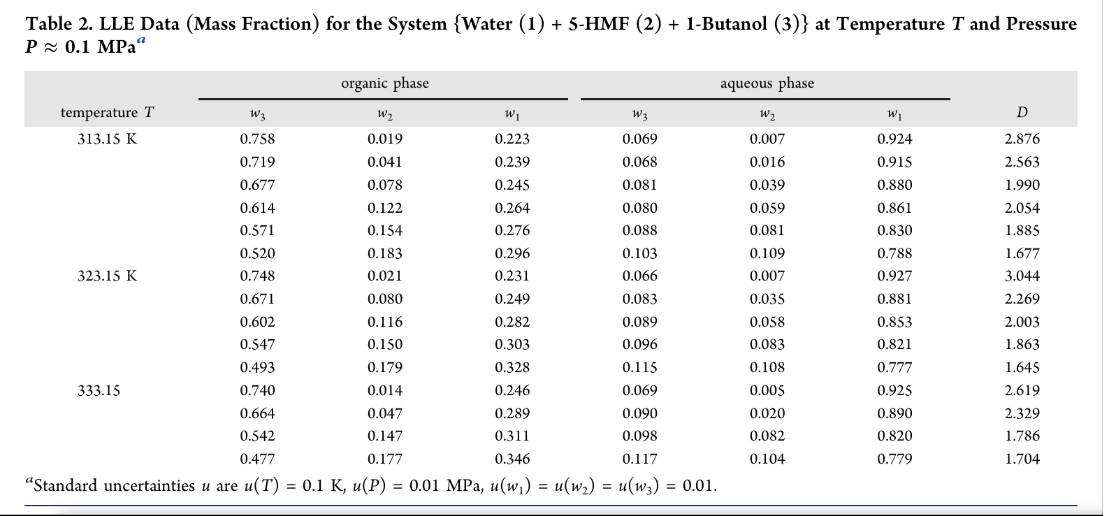
Tie lines in mole %
Convert wt % inot mol % using Molar masses (g/mol) :
MW1 = 18.015; (* Water *)
MW2 = 126.11; (* 5-HMF *)
MW3 = 74.12; (* 1-Butanol *)
MW1 = 18.015; (* Water *)
MW2 = 126.11; (* 5-HMF *)
MW3 = 74.12; (* 1-Butanol *)
Temperature = 313.15 K
x1(org) | x2(org) | x3(org) | x1(aq) | x2(aq) | x3(aq) |
0.544 | 0.0066 | 0.4494 | 0.9811 | 0.0011 | 0.0178 |
0.5696 | 0.014 | 0.4165 | 0.9799 | 0.0024 | 0.0177 |
0.5824 | 0.0265 | 0.3911 | 0.9721 | 0.0062 | 0.0217 |
0.613 | 0.0405 | 0.3465 | 0.9686 | 0.0095 | 0.0219 |
0.6319 | 0.0504 | 0.3177 | 0.9618 | 0.0134 | 0.0248 |
0.6599 | 0.0583 | 0.2818 | 0.951 | 0.0188 | 0.0302 |
Temperature = 323.15 K
x1(org) | x2(org) | x3(org) | x1(aq) | x2(aq) | x3(aq) |
0.5556 | 0.0072 | 0.4372 | 0.9819 | 0.0011 | 0.017 |
0.5879 | 0.027 | 0.3851 | 0.9722 | 0.0055 | 0.0223 |
0.6339 | 0.0372 | 0.3289 | 0.9661 | 0.0094 | 0.0245 |
0.6625 | 0.0468 | 0.2907 | 0.9589 | 0.0138 | 0.0273 |
0.6929 | 0.054 | 0.2531 | 0.9471 | 0.0188 | 0.0341 |
Temperature = 333.15 K
x1(org) | x2(org) | x3(org) | x1(aq) | x2(aq) | x3(aq) |
0.575 | 0.0047 | 0.4204 | 0.9814 | 0.0008 | 0.0178 |
0.6322 | 0.0147 | 0.3531 | 0.973 | 0.0031 | 0.0239 |
0.6706 | 0.0453 | 0.2841 | 0.9585 | 0.0137 | 0.0278 |
0.7102 | 0.0519 | 0.238 | 0.9474 | 0.0181 | 0.0346 |
In[]:=
tieLines={{{0.543972,0.0066208,0.449407},{0.981131,0.00106179,0.0178075}},{{0.569575,0.0139579,0.416467},{0.979853,0.00244762,0.017699}},{{0.582379,0.0264861,0.391135},{0.972098,0.00615427,0.0217476}},{{0.61301,0.0404677,0.346522},{0.968643,0.00948194,0.0218751}},{{0.631895,0.0503664,0.317739},{0.961806,0.0134085,0.0247851}},{{0.659935,0.0582835,0.281781},{0.950996,0.0187916,0.0302126}}}
Out[]=
{{{0.543972,0.0066208,0.449407},{0.981131,0.00106179,0.0178075}},{{0.569575,0.0139579,0.416467},{0.979853,0.00244762,0.017699}},{{0.582379,0.0264861,0.391135},{0.972098,0.00615427,0.0217476}},{{0.61301,0.0404677,0.346522},{0.968643,0.00948194,0.0218751}},{{0.631895,0.0503664,0.317739},{0.961806,0.0134085,0.0247851}},{{0.659935,0.0582835,0.281781},{0.950996,0.0187916,0.0302126}}}
(*ExtractPhase:{water,5-HMF,1-butanol}inmole%*)extractPhase=Table[tieLines[[i]][[2]],{i,1,6}];(*RaffinatePhase:{water,5-HMF,1-butanol}inmol%*)raffinatePhase=Table[tieLines[[i]][[1]],{i,1,6}];
In[]:=
ClearAll[NC,T,NTIL,xxexp,yyexp,P,z];T=313.15;data=Table[Join[extractPhase[[i]],raffinatePhase[[i]]],{i,1,Length@raffinatePhase}];
In[]:=
data
Out[]=
{{0.981131,0.00106179,0.0178075,0.543972,0.0066208,0.449407},{0.979853,0.00244762,0.017699,0.569575,0.0139579,0.416467},{0.972098,0.00615427,0.0217476,0.582379,0.0264861,0.391135},{0.968643,0.00948194,0.0218751,0.61301,0.0404677,0.346522},{0.961806,0.0134085,0.0247851,0.631895,0.0503664,0.317739},{0.950996,0.0187916,0.0302126,0.659935,0.0582835,0.281781}}
{m,n}=Dimensions[data];NC=n/2;NTIL=m;x1e=data[[All,1]];x2e=data[[All,2]];x3e=data[[All,3]];x1r=data[[All,4]];x2r=data[[All,5]];x3r=data[[All,6]];(*PHASERAFFINATE/PHASEEXTRACTforwater(1)+5-HMF(2)+1-butanol(3)ternarysystem*)xxexp={x1r,x2r,x3r};yyexp={x1e,x2e,x3e};
In[]:=
NRTL[x_]:=Module[{alp,tau,G,gam,G1,tau1,G2,s,act,aa,bb,zz,i,j},alp=Table[0.,{NC},{NC}];alp[[1,2]]=0.2;alp[[1,3]]=0.2;alp[[2,3]]=0.2;alp[[2,1]]=alp[[1,2]];alp[[3,1]]=alp[[1,3]];alp[[3,2]]=alp[[2,3]];tau=Table[P[[i,j]]/T,{i,NC},{j,NC}];G=Table[Exp[-alp[[i,j]]tau[[i,j]]],{i,NC},{j,NC}];gam=Table[0.,{NC}];G1=Table[0.,{NC},{NC}];tau1=Table[0.,{NC},{NC}];G2=Table[0.,{NC},{NC}];s=Table[0.,{NC},{NC}];Do[aa=0.;bb=0.;Do[zz=G[[j,i]]x[[j]];aa+=zz;bb+=zztau[[j,i]];,{j,NC}];gam[[i]]=bb/aa;Do[G1[[j,i]]=G[[j,i]]/aa;tau1[[j,i]]=tau[[j,i]]-gam[[i]];G2[[j,i]]=G1[[j,i]]tau1[[j,i]];s[[j,i]]=x[[i]]G2[[j,i]];,{j,NC}];,{i,NC}];Do[Do[gam[[i]]+=s[[i,j]],{j,NC}];gam[[i]]=Exp[gam[[i]]];,{i,NC}];act=Table[x[[i]]gam[[i]],{i,NC}];act]
In[]:=
EQUILIBRE[X_]:=Module[{x,y,act1,act2,f,Xt,Yt,i},x=Take[X,NC];y=Take[X,{NC+1,2NC}];act1=NRTL[x];act2=NRTL[y];f=Table[0.,{2NC+1}];Do[f[[i]]=act1[[i]]-act2[[i]],{i,NC}];Xt=Sum[X[[i]],{i,NC}];Yt=Sum[X[[i]],{i,NC+1,2NC}];f[[NC+1]]=1-Xt;f[[NC+2]]=1-Yt;Do[f[[NC+2+i]]=z[[i]]-X[[i]]X[[2NC+1]]-X[[i+NC]](1-X[[2NC+1]]),{i,NC-1}];f]
Part B: LLE diagram computation using common tangent plane and arc - length continuation
Part B: LLE diagram computation using common tangent plane and arc - length continuation
Method based on common tangent plane and arc - length continuation
NRTL Model Parameters at T=298.15 K from my above hybrid optimization code and stored in P
tau_ij for water (1) + 5-HMF (2) + 1-butanol (3)
Alpha matrix (symmetric)
Composition vector
NRTL activity coefficients
Dimensionless Gibbs energy of mixing: g/RT
Derivatives
Unknowns
Common tangent equations
Extra constraint - Prevent trivial solution xα=xβ
First value for d --- very small d=0.0001 yield approximately the plait point
First value for d --- very small d=0.0001 yield approximately the plait point
Solution is near {0.56,0.04}
Type I liquid-liquid equilibrium (LLE) diagram - Plait point indicated in red
Figure and Table from Ref . 2
water-rich phase {x1,x2,x3}, org-rich phase {x1,x2,x3}
Display as tables with headers
Combine into tie-line pairs:{phaseI,phaseII}
Show all nine experimental tie lines
Let us compute the RMSD