These are called Borwein integrals, after David and Jonathan Borwein, the father-and-son mathematicians who first presented them in their paper: Borwein, David; Borwein, Jonathan M. (2001), “Some remarkable properties of sinc and related integrals”, The Ramanujan Journal, 5 (1): 73–89. https://doi.org/10.1023%2FA%3A1011497229317
Engineer Hanspeter Schmid writes, “[W]hen this fact was recently verified by a researcher using a computer algebra package, he concluded that there must be a ‘bug’ in the software. It is not a bug, though; this series of integrals really only results in π/2 up to a certain point, and then breaks down. This astonishes most mathematically educated readers, as especially those readers mentally extrapolate the sequence shown above and find it surprising that something fundamental should change when the factor sinc(x/15) is introduced.” He gives a graphic explanation of what’s happening in the paper: Schmid, Hanspeter (2014), “Two curious integrals and a graphic proof” (PDF), Elemente der Mathematik, 69 (1): 11–17. https://doi.org/10.4171%2FEM%2F239
Problem statement
Problem statement
Check out this strange behavior:
In[]:=
∞
∫
0
Sin[x]
x
Out[]=
π
2
In[]:=
∞
∫
0
Sin[x]
x
Sin[x/3]
x/3
Out[]=
π
2
In[]:=
∞
∫
0
Sin[x]
x
Sin[x/3]
x/3
Sin[x/5]
x/5
Out[]=
π
2
In[]:=
∞
∫
0
Sin[x]
x
Sin[x/3]
x/3
Sin[x/5]
x/5
Sin[x/7]
x/7
Out[]=
π
2
In[]:=
∞
∫
0
Sin[x]
x
Sin[x/3]
x/3
Sin[x/5]
x/5
Sin[x/7]
x/7
Sin[x/9]
x/9
Out[]=
π
2
In[]:=
∞
∫
0
Sin[x]
x
Sin[x/3]
x/3
Sin[x/5]
x/5
Sin[x/7]
x/7
Sin[x/9]
x/9
Sin[x/11]
x/11
Out[]=
π
2
In[]:=
∞
∫
0
Sin[x]
x
Sin[x/3]
x/3
Sin[x/5]
x/5
Sin[x/7]
x/7
Sin[x/9]
x/9
Sin[x/11]
x/11
Sin[x/13]
x/13
Out[]=
π
2
In[]:=
∞
∫
0
Sin[x]
x
Sin[x/3]
x/3
Sin[x/5]
x/5
Sin[x/7]
x/7
Sin[x/9]
x/9
Sin[x/11]
x/11
Sin[x/13]
x/13
Sin[x/15]
x/15
Out[]=
467807924713440738696537864469π
935615849440640907310521750000
This is quite close to π€/2:
In[]:=
N[%]-
π
2
Out[]=
-2.31006×
-11
10
The next term in the series is a little farther away from π€/2:
In[]:=
∞
∫
0
Sin[x]
x
Sin[x/3]
x/3
Sin[x/5]
x/5
Sin[x/7]
x/7
Sin[x/9]
x/9
Sin[x/11]
x/11
Sin[x/13]
x/13
Sin[x/15]
x/15
Sin[x/17]
x/17
Out[]=
17708695183056190642497315530628422295569865119π
35417390788301195294898352987527510935040000000
In[]:=
N[%]-
π
2
Out[]=
-1.87245×
-8
10
It only gets worse from there:
In[]:=
∞
∫
0
Sin[x]
x
Sin[x/3]
x/3
Sin[x/5]
x/5
Sin[x/7]
x/7
Sin[x/9]
x/9
Sin[x/11]
x/11
Sin[x/13]
x/13
Sin[x/15]
x/15
Sin[x/17]
x/17
Sin[x/19]
x/19
Out[]=
8096799621940897567828686854312535486311061114550605367511653π
16193600755941299921751838065715269433640150152124763150000000
In[]:=
N[%]-
π
2
Out[]=
-1.46671×
-7
10
What’s going on here?
Analysis
Analysis
Each integral is a product of scaled sinc functions, which corresponds to a convolution of scaled rect functions in the Fourier domain.
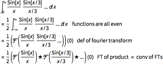
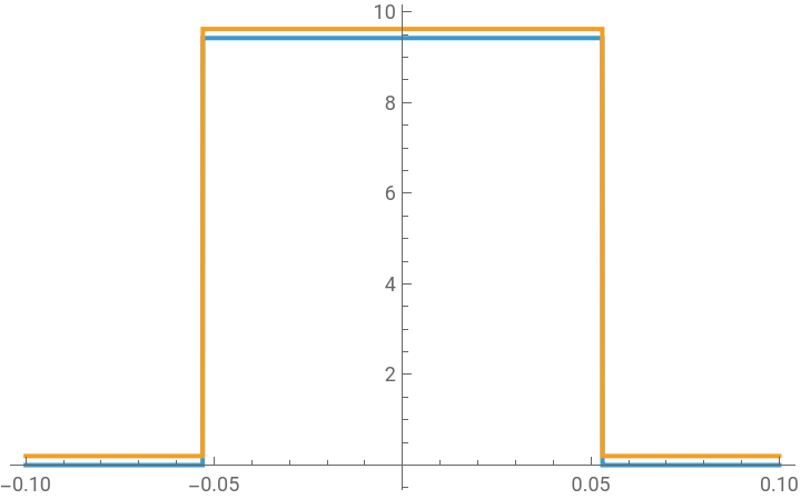
Next we use the fact that the FT of a sinc is a rect. Specifically:

Example:
c=3;ft=FourierTransform,x,s,FourierParameters->{0,-2π}/.s->x;box=cπUnitBox[cπx];Plot{ft,.2+box},{x,-.1,.1},
Sin[x/c]
x/c
Out[]=


So our integral becomes
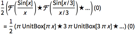
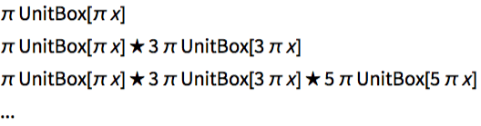
We now study the series of convolutions π UnitBox[π x]★ 3π UnitBox[3π x]★ ...
The UnitBoxes:
cs=Range[1,9,2];boxes=Table[πcUnitBox[πcx],{c,cs}];Plotboxes,{x,-.2,.2},
Out[]=
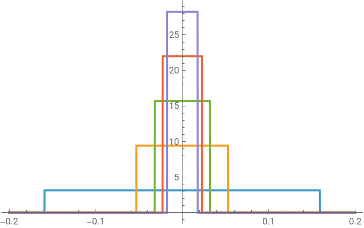


They all have unit area:
In[]:=
∞
∫
-∞
Out[]=
{1,1,1,1,1}
The boxes’€™ widths follow a simple pattern as they get smaller:
In[]:=
centerWidth[box_]:=ArcLength@ImplicitRegion[Reduce[box==(box/.x->0)],{x}]centerWidth/@boxes
Out[]=
,,,,
1
π
1
3π
1
5π
1
7π
1
9π
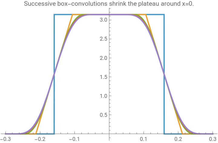
Convolving these boxes together yields a progressively smoother function.
Here is the succession of convolutions
In[]:=
convs=FoldList[(Convolve[#1,#2,x,s]/.s->x)&,boxes];
Plotconvs,{x,-.3,.3},
Out[]=
Zoom in:
At 0, each convolution takes the value π:
However, successive convolutions’ widths get smaller:
Does this sequence stay positive forever, or does it cross zero?
Brute-force find a pattern:
So it looks like the x/15 term has a “negative” width, indicating the plateau has been convolved away.
Besides this weird formula with harmonic numbers, there is a simpler way to express the widths of the convolutions. Convolving a box with a smaller box of width c reduces the width of the flat center region by c. So the width of successive box-convolutions can be found by successively subtracting box widths from the width of the original box 1/π:
This matches the widths we found with symbolic convolution:
This is good because the closed-form expression of the x/15 convolution is too big for Mathematica.
This matches the widths of our symbolic convolutions, as well as our werd formula with harmonic numbers:
CITE THIS NOTEBOOK
CITE THIS NOTEBOOK
Borwein Integrals: UnitBox spectral depletion and the mechanism of integral deviation
by Justin Pearson
Wolfram Community, STAFF PICKS, May 12, 2026
https://community.wolfram.com/groups/-/m/t/3715139
by Justin Pearson
Wolfram Community, STAFF PICKS, May 12, 2026
https://community.wolfram.com/groups/-/m/t/3715139