Nullcline Plot

′

x

(t) =

y

(y-1.5x)

2

x

+

2

y

-9

(y-0.25)

2

x

+y-2

′

y

(t) =

2x+

2

y

-1

-x-2y+1

1.51-

2

x

y-x

solution

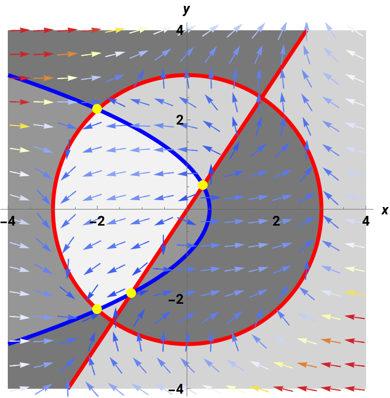
A nullcline plot for a system of two nonlinear differential equations provides a quick tool to analyze the long-term behavior of the system. The

x

and

y

nullclines (

x'=0

,

y'=0

) are shown in red and blue, respectively. The nullclines separate the phase plane into regions in which the vector field points in one of four directions: NE, SE, SW, or NW (indicated here by different shades of gray). The equilibrium points of the system are the points of intersection of the two kinds of nullclines. Hovering over an equilibrium point displays a tooltip with the eigenvalues of the linearization of the system at that point.

Details

Displaying a solution with its initial value at the locator is optional.

References

[1] P. Blanchard, R. L. Devaney, and G. R. Hall, Differential Equations, 4th ed., Boston: Brooks–Cole, 2010 pp. 478ff.

Permanent Citation

Helmut Knaust

"Nullcline Plot"
http://demonstrations.wolfram.com/NullclinePlot/
Wolfram Demonstrations Project
Published: December 6, 2013