ABSTRACT (original article): We find a quartic example of a smooth embedded negatively curved surface in homeomorphic to a doubly punctured torus. This constitutes an explicit solution to Hadamard’s problem of constructing complete surfaces with negative curvature and Euler characteristic in . Further we show that our solution has the optimal degree of algebraic complexity via a topological classification for smooth cubic surfaces with a negatively curved component in : any such component must either be topologically a plane or an annulus. In particular we prove that there exists no cubic solutions to Hadamard’s problem. CITATION (original article): Connell, Chris and Ghomi, Mohammad. “Topology of negatively curved real affine algebraic surfaces” Journal für die reine und angewandte Mathematik, vol. 2008, no. 624, 2008, pp. 1-26. https://doi.org/10.1515/CRELLE.2008.078
3
ℝ
3
ℝ
3
ℝ
This notebook is an accompaniment to the paper Topology of negatively curved real affine algebraic surfaces by Chris Connell and Mohammad Ghomi. Here we verify that the following equation
eq=3+2(1+4xy)-2+8xy-1==0;
4
z
2
z
2
(+)
2
x
2
y
gives a complete negatively curved surface Σ in which is homeomorphic to a doubly punctured torus. This yields an explicit algebraic solution to a problem first studied by Hadamard.We also study the projective transformations of this equation which yield some surfaces with nonpositive curvature. Finally, we obtain a sharp estimate for the merging of two hyperboloids to be negatively curved.
3
R
Defining the Hessian and figure of Σ
Defining the Hessian and figure of Σ
DetHess[f_][x_,y_]:=D[f[u,v],u,u]D[f[u,v],v,v]-/.{ux,vy};
2
D[f[u,v],u,v]
Figure of Σ
Figure of Σ
ContourPlot3D[eq//Evaluate,{x,-3,3},{y,-3,3},{z,-1.5,1.5},PlotPoints{30,30,20},BoxRatiosAutomatic,AxesFalse]

Regularity of Σ
Regularity of Σ
Here we check that our main surface in regular. To see this note that our surface is given by (-1)where
-1
F
F[x_,y_,z_]:=2-2-3-8xy(1+)
2
(+)
2
x
2
y
2
z
4
z
2
z
So we just need to check that -1 is a regular value of F:
gradF:={F[x,y,z],F[x,y,z],F[x,y,z]}
∂
x
∂
y
∂
z
gradF//FullSimplify
{8(+x-y(1+)),8(y+-x(1+)),-4(z+4xyz+3)}
3
x
2
y
2
z
2
x
3
y
2
z
3
z
Thus for the gradient to vanish we must have z=0.
gradF/.{z0}
{-8y+8x(+),-8x+8y(+),0}
2
x
2
y
2
x
2
y
Solve[{-8y+8x(+),-8x+8y(+)}{0,0}]
2
x
2
y
2
x
2
y
{x0,y0},x-,y-,x-,y,x,y-,x,y
1
2
1
2
2
2
2
2
1
2
1
2
F[0,0,0]
0
F-,-,0
1
2
1
2
-2
F,,0
1
2
1
2
-2
So the only singular values are 0, and -2.
Curvature of Σ
Curvature of Σ
There are two cases to consider:
Case I: z ≠ 0
Case I: z ≠ 0
Case II: z = 0
Case II: z = 0
R[θ_]:=
Cos[θ] | -Sin[θ] |
Sin[θ] | Cos[θ] |
R.
π
4
x |
y |
-,+
x
2
y
2
x
2
y
2
1+2==2+3+8xy(1+)/.x->-,y->+//FullSimplify
2
(+)
2
x
2
y
2
z
4
z
2
z
x
2
y
2
x
2
y
2
1+2+2+4(-1+-)+4(1+)2+3
4
x
4
y
2
x
2
y
2
z
2
y
2
z
2
z
4
z
1+2+2+4(-1+-)+4(1+)2+3/.{z0}
4
x
4
y
2
x
2
y
2
z
2
y
2
z
2
z
4
z
1+2+4+2+4(-1+)0
4
x
2
y
4
y
2
x
2
y
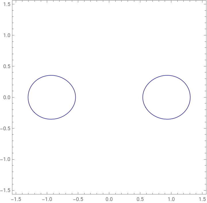
Here is the picture of the intersection of the surface with the xy-plane.
ContourPlot1+2+4+2+4(-1+)0,{x,-1.5,1.5},{y,-1.5,1.5},AxesOrigin{0,0},Ticks{{-1,1},{-1,1}},AxesLabel{"x","y"}
4
x
2
y
4
y
2
x
2
y
1+2+4+2+4(-1+)0/.{y0}
4
x
2
y
4
y
2
x
2
y
1-4+20
2
x
4
x
Solve[%,x]
x-(2-,x(2-,x-(2+,x(2+
1
2
2
)1
2
2
)1
2
2
)1
2
2
)N[%]
{{x-0.541196},{x0.541196},{x-1.30656},{x1.30656}}
Case I. 1 y ≠ 0
Case I. 1 y ≠ 0
Solve[1+2+2+4(-1+-)+4(1+)2+3,y]
4
x
4
y
2
x
2
y
2
z
2
y
2
z
2
z
4
z
y-,y
-1--+
,y2
x
2
z
1+8+6+8+5
2
x
2
z
2
x
2
z
4
z
2
-1--+
,y-2
x
2
z
1+8+6+8+5
2
x
2
z
2
x
2
z
4
z
2
-2-2-2-
2
x
2
z
2
1+8+6+8+5
2
x
2
z
2
x
2
z
4
z
2
-2-2-2-
2
x
2
z
2
1+8+6+8+5
2
x
2
z
2
x
2
z
4
z
2
f[x_,z_]:=
-1--+
2
x
2
z
1+8+6+8+5
2
x
2
z
2
x
2
z
4
z
2
DetHess[f][x,0]//FullSimplify
-42+2813+6-3
2+16
-162
x
2
x
2
x
2+16
2
x
2
(1+8)
2
x
2
-2-2+
2
x
2+16
2
x
Numerator[%]--42-208-96+4)//Simplify
2
x
4
x
2+16
(7+122
x
2
x
0
2
(-42-208-96)
2
x
4
x
2
4)
2+16
(7+122
x
2
x
196-448+3712+3072+9216
2
x
4
x
6
x
8
x
Solve[%==0,x]//N
{{x-0.453562+0.67507},{x0.453562-0.67507},{x-0.453562-0.67507},{x0.453562+0.67507},{x-0.389752+0.261864},{x0.389752-0.261864},{x-0.389752-0.261864},{x0.389752+0.261864}}
Case I. 2 y = 0
Case I. 2 y = 0
Solve[1+2+2+4(-1+-)+4(1+)2+3,x]
4
x
4
y
2
x
2
y
2
z
2
y
2
z
2
z
4
z
x-
1-+-
,x2
y
2
z
1-8+6-8+5
2
y
2
z
2
y
2
z
4
z
2
1-+-
,x-2
y
2
z
1-8+6-8+5
2
y
2
z
2
y
2
z
4
z
2
1-++
,x2
y
2
z
1-8+6-8+5
2
y
2
z
2
y
2
z
4
z
2
1-++
2
y
2
z
1-8+6-8+5
2
y
2
z
2
y
2
z
4
z
2
Projective Transformations of Σ
Projective Transformations of Σ
First we are going to rotate the surface as this will make performing the projective transformations easier:
So our new equation will be:
Punctured Torus
Punctured Torus
Solve[eq2/.{y->0,z->0},x]
Triply Punctured Sphere
Triply Punctured Sphere
Solve[eq2/.{x->0, y->0},z]
Doubly punctured sphere
Doubly punctured sphere
Solve[eq2/.{z->0, x->1},y]
We switch y and z for better visualization:
Flat Points of the Projective Transformations
Flat Points of the Projective Transformations
All projective transformations of Σ necessarily have nonpositive curvature; however, in general they are not negatively curved, since they may pick up flat points along the planes which were blown up during the projective transformation.
Punctured Torus
Punctured Torus
First recall that the equation for this surface is
Note that we switched x and z. This is so that it can be visualized better once we graph it.
Triple Punctured Sphere
Triple Punctured Sphere
First recall that the equation for this surface is given by:
Here we check that this equation can be rewritten more simply as follows:
It appears that the real roos are the thirs and fourth roots which are the same up to a sign.
Doubly Punctured Sphere
Doubly Punctured Sphere
First recall that the equation for this surface is given by:
Here we check that this equation can be rewritten more simply as follows:
How the Equation for Σ Was Obtained
How the Equation for Σ Was Obtained
The main idea here was to work with "Cassini Ovals". These are the loci of points in the plane whose product of distances from a pair of given points is constant. For instance consider:
Our formula is just the numerator of the above:
The most difficult part was to adjust the rate of scaling of the ovals with the rate of vertical shifting to make sure that the curvature remains negative.
Sharp Estimate for MergingTwo Hyperboloids
Sharp Estimate for MergingTwo Hyperboloids
Figure
Figure
Negatively Curved Surfaces in a Slab
Negatively Curved Surfaces in a Slab
CITE THIS NOTEBOOK
CITE THIS NOTEBOOK
Topology of negatively curved real affine algebraic surfaces
by Chris Connell & Mohammad Ghomi
Wolfram Community, STAFF PICKS, January 22, 2025
https://community.wolfram.com/groups/-/m/t/3362048
by Chris Connell & Mohammad Ghomi
Wolfram Community, STAFF PICKS, January 22, 2025
https://community.wolfram.com/groups/-/m/t/3362048